Guaranteed Income and Optimal Retirement Glide Paths

Journal of Financial Planning: June 2024

Executive Summary

• Deciding on asset allocations over time and portfolio withdrawal rates remain key considerations for retirees. These decisions are impacted by factors such as the investor’s wealth level, degree of risk aversion, the desire to leave a bequest, and the presence of guaranteed income, such as Social Security. This paper considers these issues as they relate to utility levels for retirees. 
• Initial equity allocations from 0 to 100 percent were examined. For investors with moderate and high levels of risk aversion, higher proportions of Social Security relative to overall wealth led to higher initial optimal allocations to stock. This is somewhat intuitive because the higher level of guaranteed income allows for more risk with the remainder of the portfolio. However, retirees who rely more on Social Security are less wealthy, and lower levels of wealth are generally equated with lower allocations to stock.
• Five different glide paths, which provide plans for changes in allocations to stocks over time, were considered: increasing the weight of stock slowly, increasing fast, decreasing slowly, decreasing fast, and constant. The typical guidance for retirees is to decrease their allocation to stock over time. This paper finds, however, that increasing glide paths, where the level of stock increases over time, are often optimal. 

Doug Waggle is a professor of finance in the College of Business at the University of West Florida. He teaches courses in financial planning and investments. He earned his Ph.D. in finance from the University of Alabama and his M.B.A. from the University of Southern Mississippi.

Pankaj Agrrawal is the Nicolas M. Salgo professor of finance at the University of Maine. He earned his Ph.D. in finance from the University of Alabama, after which he worked in the asset management industry for about a decade.
 

NOTE: Click on the Tables and Equations below for clearer PDF versions.

JOIN THE DISCUSSION: Discuss this article with fellow FPA Members through FPA's Knowledge Circles​​​​. ​​​

FEEDBACK: If you have any questions or comments on this article, please contact the editor HERE. 

Retirees are faced with many decisions in their quests to achieve lifetime income from their portfolios. Two of the biggest financial choices they must make are deciding on their portfolio glide paths (altering their asset allocation with the passage of time) and the size of the withdrawals they should make from those portfolios. The mix of stocks and bonds in the portfolio is a primary driver of success, where success is defined as providing predictable income that at least keeps up with inflation for the life of the retiree. Investing too safely, with a high percentage of bonds, might mean trailing inflation and a declining standard of living. Investing more aggressively, however, might result in a large drop in wealth early in retirement with no time or potential future income to make it up. Deciding on how much to withdraw from the portfolio is another Goldilocks situation. If portfolio withdrawals to fund retirement income are too low, the utility from underutilized spending power is lost forever. Conversely, if the portfolio withdrawals are too high, retirees face the risk of running out of money before they die. 

Target retirement date funds, which change their asset allocations over time, would seem like a good way for retirees to put their portfolios on autopilot and let the fund managers deal with at least the glide path issue. Unfortunately, there is no one-size-fits-all retirement plan available. Some retirees may be comfortable with taking on more risk to get a 5 percent withdrawal rate, while others may like the relative security of a 3 percent withdrawal rate, despite the considerably lower payouts. That means that the choice of the withdrawal rate itself could impact the asset allocation / glide path decision. Retirees planning on higher withdrawal rates might need higher allocations to stock over time to get a successful outcome. There are other reasons why the retirement portfolio planning process is individualized. Individual retirees have different risk aversion levels, so not everyone would be comfortable with the same portfolio guidance. Retirees also have different levels of guaranteed income, such as Social Security payments or pensions, that allow them to rely less on their portfolio performance. Going beyond the issue of lifetime income, some retirees may also want to provide bequests to heirs or charities after they die, which could also drive portfolio decisions.

This paper utilized Monte Carlo simulations to examine the important issues noted above. Cases were included where retirees have different levels of (1) risk aversion, (2) desire as far as bequests, and (3) guaranteed income, such as Social Security payments. The paper investigated the impact of these three items on overall investor utility and ultimately on making optimal portfolio decisions. Retirees were assumed to invest in a combination of stocks and bonds that they rebalanced in a planned fashion on an annual basis. A wide range of initial allocations to stock, with up to five possible glide paths each, were considered. This paper built on earlier works to illustrate the impact of guaranteed income on retiree portfolio decisions. 

Literature Review 

There have been many papers on safe withdrawal rates since Bengen (1994) first developed the widely cited 4 percent rule. The 4 percent rule suggests that retirees can safely withdraw that amount from their initial portfolio balance in the first year of retirement and subsequently adjust their annual withdrawal amounts to keep up with inflation. This assumes a roughly 30-year planned retirement in conjunction with an appropriate portfolio. Bengen (1994) supported this finding using historical data assuming different fixed allocations to a portfolio of stock and bonds, and he recommended a starting allocation of 50 to 75 percent stocks. Cooley, Hubbard, and Walz (2011) suggested drawing the “line” at a 75 percent chance of success for client portfolios, meaning that strategies with this probability of succeeding based on historical data should be a reasonable starting point for financial planning clients. Requiring a higher success rate would necessitate lower withdrawal rates (and a lower standard of living) for retirees. Cooley, Hubbard, and Walz (2011) also supported withdrawal rates in the 4 to 5 percent range for retirees wanting annual inflation increases, assuming portfolio allocations of at least 50 percent stock.

Pfau (2011) argued that the 4 percent rule may not work, depending on market valuations and bond yields present at the time an individual retires. Bond yields in the United States were trapped at historically low rates for many years, and papers such as Finke, Pfau, and Blanchett (2013), Blanchett, Finke, and Pfau (2013), Blanchett (2015), and Waggle, Moon, and Lee (2022) addressed how this situation would impact retirement portfolios. Waggle, Moon, and Lee (2022) determined that a low interest rate environment favored higher allocations to stock that decreased over time as rates returned to normal. Market interest rates have increased considerably since these papers were published, with the federal funds rate increasing from 0.25 percent in March 2022 to 5.25–5.50 percent in December 2023.¹ 

There have also been papers that included the impact of guaranteed income, such as Social Security payments, in their analysis. Finke, Pfau, and Williams (2012) examined the case of a retired couple with a $1 million nest egg and either $20,000 or $60,000 per year in guaranteed income. They considered fixed stock allocations and various withdrawal rates and concluded that the extra $40,000 in guaranteed income allowed for a 1 percent increase in the safe withdrawal rate. Blanchett (2017) also found that guaranteed income had a significant impact on safe withdrawal rates. Blanchett and Finke (2018) found that purchasing income annuities should lead to retirees taking on more risk (higher allocations to stock) with their remaining portfolio balance. This means that annuities should generally be purchased from bond funds, rather than stock, since the guaranteed payouts of annuities are similar to the cash flows of bonds.

Glide paths in retirement, where the asset allocation changes over time in a predetermined fashion, have also been a topic of conversation. Blanchett (2007) assumed that stocks and bonds performed at their long-term averages and found that constant stock allocations were the best portfolio option in most cases. Spitzer and Singh (2008) likewise found that constant stock allocations outperformed glide paths where the allocation to stock slowly decreased over time. Kitces and Pfau (2015) concluded that when equity markets were considered overvalued, glide paths with increasing stock allocations over time are preferred. When Blanchett (2015) incorporated a low interest rate environment into his study, glide paths with declining allocations to stock were favored. Waggle, Moon, and Lee (2022) looked at multiple scenarios for low interest rates returning to normal and also supported decreasing allocations to stock over time. Pfau and Kitces (2014), with assumptions that interest rates were in a more normal range, tested a whole range of beginning and ending stock allocations and found that rising glide paths maximize sustainable retirement income.

The current paper adds to several of these earlier works. While Finke, Pfau, and Williams (2012) examined the impact of guaranteed income on overall utility and portfolio decisions, they only considered portfolios with constant allocations. The current paper extends this by considering constant, increasing, and decreasing glide paths. In addition, this paper also provides a comparison of how portfolio utility rankings would look with and without guaranteed Social Security payments considered. Blanchett (2015) and Blanchett (2017) considered glide paths and the impact of guaranteed income, respectively, but both of these papers were products of a low-interest-rate environment. Bond rates were at historically low levels during that period, so both works assumed that bond rates would start low and increase over time. Rates have increased since then, and that is reflected in the current paper. Pfau and Kitces (2014) argued in favor of increasing allocations to stock during retirement, but they focused only on success rates. This paper included both success rates and glide path ranks based on utility preferences of the investors. 

Glide Paths 

Glide paths show investors’ planned asset allocation changes over time. For this paper, it was assumed that portfolios were allocated between a mix of 10-year Treasury bonds and a diversified portfolio of large-cap stock, such as the Standard and Poor’s 500 Index. While other asset categories could have been included, large company stocks and (Treasury and/or corporate) bonds are typical core portfolio elements. Including just stocks and bonds allowed the analysis to easily focus on differing stock levels. A portfolio of 60 percent stock and 40 percent bonds is often noted as providing a good balance of risk and return for investors seeking a mix of growth and income, but the general guidance for retirees tends to be to gradually decrease portfolio allocations to stock over time.² Short selling was not allowed in the analysis, so stock and bond levels could not go below zero.

One example of a glide path is exemplified by the common rule of thumb, which suggests that the percentage of stock in an investor’s portfolio should equal 100 minus their age. Following this guidance, a 67-year-old investor would start with 33 percent of their financial assets in stock and decrease this by 1 percent each year. By age 100, should they live that long, that investor would have 100 percent of their portfolio in bonds and no money in stock. A somewhat more aggressive version of this rule is to allocate 110 minus the investor’s age to stock. 

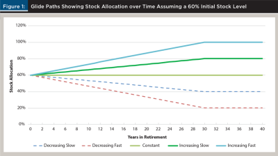
This paper presents initial allocations to stock of between 0 and 100 percent in 10-percent increments. For each of these beginning stock levels, up to five possible glide paths were considered: (1) decreasing slow, (2) decreasing fast, (3) constant, (4) increasing slow, and (5) increasing fast. The portfolio rebalancing in each of the glide paths occurred at the end of each year. So, at the end of each year, the stock and bond levels were reset according to the different glide paths. These glide paths were comparable to Blanchett (2015), except that the changes in asset allocations for all of the glide paths, other than the constant case, occurred over 30 years, rather than 40 years. Since this work assumed retirement at age 67, as noted below, a 40-year glide path would not be relevant for most retirees. After 30 years, the glide paths were all held constant at their 30-year asset mixes. For the decreasing slow paths, the allocation to stock decreased in equal percentage increments by a total of 20 percent over 30 years while the total 30-year reduction was 40 percent in the decreasing fast paths. Likewise, the increasing slow and increasing fast paths had 20 and 40 percent total increases in stock allocations, respectively, over 30 years. In the constant glide paths, portfolios were rebalanced to their initial levels at the end of each year.

Clearly, not all the glide paths are possible from each of the starting stock allocations. If the full 30-year change of 20 or 40 percent, decreasing or increasing, was not possible, that particular path was not considered. For example, from a starting portfolio allocation of 0 percent stock, decreasing positions are not possible without short selling, so only the constant, increasing slow, and increasing fast models were considered. With an initial stock allocation of 20 percent, the decreasing slow path is an option, while the decreasing fast path is not. Figure 1 shows the tracks of the five glide paths considered assuming a 60 percent initial stock allocation. As noted above, all of the paths leveled out after 30 years, and the simulations ended after 40 years. Based on these guidelines, a total of 43 different initial stock level / glide path options were considered.

Mortality and Social Security

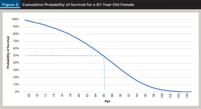
The relevant retirement period to plan for depends on factors such as the retiree’s life expectancy and tolerance for risk. Healthier individuals should likely plan for longer retirement time horizons than unhealthy individuals. As a general guideline, the Society of Actuaries (SOA) mortality tables for 2012 suggest that a female retiring at age 67 has about a 50 percent chance of surviving to about age 86, while a male retiring at the same age would have only about a 42 percent chance of living that long. That same female would have only about a 10 percent chance of living to age 97 compared to just a 5 percent chance for the male. Of course, with a couple, the odds of at least one member of the pair surviving to a certain age are higher. The SOA data is used by actuaries to price products such as annuities, which are more likely to be purchased by healthier individuals who are expected to live longer. Figure 2 shows the cumulative probability of survival, Survival_t, for a 67-year-old female.

Everything else equal, the longer a retiree’s expected lifespan, the more valuable guaranteed Social Security payments are to them. The value of Social Security to a 67-year-old female at the beginning of retirement is estimated by finding the present value of the expected payouts over the next 40 years.³ This differs somewhat from finding the value of a bond, for example, because the expected payouts must also consider the probability of surviving to receive those payments. With a 40-year bond, payments are guaranteed for the full term. However, for a single retiree on Social Security, the payments end if the retiree dies. This could be after one year or after 40 or more years. Most retirees will not receive benefits for anywhere near 40 years, though. 

Equation 1 was used to find the initial value of the expected Social Security payments at age 67 SS₀:

(1)

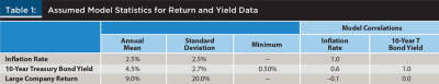
where SSI_t is the Social Security income at time t and COLA_t is the cost-of-living adjustment based on the prior year’s rate of inflation. Given that the individual was alive at age 67, their probability of survival to a particular age is given by Survival_t, as noted in the discussion of mortality above. The expected value of each future payment was discounted back to current dollars based on the zero-coupon yield curve rate for that length of time, r_t. The initial yield curve assumptions were based on the assumed long-term average nominal rates for 1-year Treasury bills, 10-year Treasury bonds, and 20-year Treasury bonds of 3.7 percent, 4.5 percent, and 4.7 percent, respectively. The initial COLA assumption was that inflation would stay at the assumed average of 2.5 percent, as given in Table 1.

After finding the beginning value of Social Security for the retiree with equation 1, portfolios with various levels of financial assets (stock and bonds) relative to the value of Social Security were considered as part of the analysis described below. Results were presented for cases where stocks and bonds were one-third, two times, and five times the initial value of Social Security. This translates to having cases where Social Security was 75 percent, 33 percent, and 17 percent of overall wealth, respectively.⁴

Simulations 

This study considered the case of a single female who retires at age 67, the full retirement age for those who turn 62 in 2023 or later, and collects income from both a portfolio of stocks and bonds and Social Security payments. The analysis was simplified by looking at the case of a single retiree, rather than a couple, so that there were no confounding issues such as different income levels and survivor benefits to consider.⁵ Accordingly, the life expectancy numbers for females, which are somewhat higher than those of males, were used in the mortality calculations. 

The process in the simulations followed the portfolio actions that would be taken by a retiree over the assumed 40-year retirement period. First, a desired payout level and a planned glide path for the portfolio were selected. With a payout level, such as the commonly cited 4 percent, the retiree took that percentage of their stock–bond portfolio as income in the first year of retirement. Each year thereafter the dollar amount of the planned withdrawal was increased by the (simulated) rate of inflation to keep the retiree’s income constant in real terms. Likewise, the individual’s initial annual Social Security payment was also increased with inflation each year. The retiree was assumed to have collected income from both their stock–bond portfolio (as long as it maintained a positive balance) and a Social Security payment. The portfolio balance was adjusted each year based on simulated market returns for stocks and bonds. At the end of each year, the retirement portfolio was rebalanced following the prescribed glide path. A total of 1,000 simulations were run for each combination of payout level and glide path. Once the simulations were completed, the success rates and average utility of each combination were measured, as described in separate sections below.

Specific details on the Monte Carlo simulation used to model annual inflation, 10-year Treasury bond (bonds) yields and total returns, and large-company stock (stock) total returns are described below. Table 1 presents the assumed long-term means of the returns and yields, along with the standard deviations and correlations of those factors. While the correlations of inflation, stock, and bond yields were based on long-term (1970–2022) historical averages, the return and yield figures used are more conservative than what long-term history would suggest. The use of an inflation rate and bond yield lower than what was observed during that period was a concession to the power of the Federal Reserve. The Federal Reserve has had an implicit average inflation target of 2 percent since 1996 that it made formal in 2012.⁶ That 2-percent target is still in place and remains an ongoing point of discussion in the financial press. While 2 percent was the target from 1996 to 2022, inflation actually averaged about 2.5 percent during that period, which is what was assumed in the analysis. Since bond yields (rather than total returns) are highly correlated with inflation, the lower inflation target would tend to imply lower yields as well. A total of 1,000 possible outcomes for stocks, bonds, and inflation over 40 years were generated. These scenarios provided the asset returns that were used to test the performance of the various glide paths, withdrawal rates, and wealth levels.

Overall price levels and stock values, which generate inflation and stock return numbers, respectively, were modeled using the geometric Brownian motion process (GBM). With GBM, prices or values are assumed to follow a random normal distribution. The next value in the process depends on the current value, but there is no other memory of the path. This is the basis of the “random walk” nature of stock prices. The distribution of stock returns in the long run appears to be more lognormal in nature because stock prices have a floor value of $0, while their upside potential is unlimited. Despite this, the normal distribution does a reasonably good job of modeling stock prices in the short run. Equation 2 captures GBM in discrete time and was used to model the index levels over time S_t for both stock and inflation:

(2)
 

The continuously compounded return and the standard deviation of the percentage changes in the index are shown as r and s, respectively. The change in time is dt, which is 1 when annual returns are considered. The random nature of the path over time is captured by z, which is a random normal variable with a mean of 0 and a standard deviation of 1. 

Inflation rates based on the changes in the index level derived from equation 2 were used to adjust Social Security payments and desired stock–bond portfolio withdrawals each year in the simulations. Consistent with the Social Security Administration’s handling of payment calculations, if inflation was negative in a given year (reflected by a decline in the inflation index), the following year’s Social Security payment (and planned withdrawal from the stock–bond portfolio) stayed unchanged. However, there were no subsequent increases in payments until the overall inflation index level went back above its prior high.

While the movements of stock prices appear to be random, current bond yields are highly dependent on their prior levels. Bond yields are also considered to have a long-term tendency to revert to the mean, but that force is relatively weak, as evidenced by the long period of extremely low interest rates seen in the United States from 2012 to 2021. Bond yields over time were modeled with the widely used Cox, Ingersoll, and Ross (1985) (CIR) methodology shown in equation 3:

(3)
 

Bond yields at a point in time are given by y_t, and ȳ is the long-term average yield of the 10-year Treasury bond. The overall tendency to revert to the mean is driven by the reversion factor rev, and it gets stronger the further yields get from their long-term averages (ȳ – y_t–1). One strength of the CIR model is that it recognizes that the variability of yields increases as interest rates rise, and vice versa. This means that if market yields are at 10 percent, the potential variability is much higher than if rates are at 1 percent. This changing variability is captured in the model where the standard deviation of the yields is multiplied by the square root of the prior period’s yield,  . The higher the prior period’s yield, the higher the potential variability.

One additional adjustment to the bond yields calculated with equation 3 was needed to ensure that all of the simulated yields were positive. For each period, the result was the maximum of either the calculated yield forecast or the assumed minimum yield of 0.5 percent. While some other countries have courted negative interest rates,⁷ the Federal Reserve has never shown any desire for that counterintuitive outcome in the United States. 

Positive bond yields, of course, do not mean that bond total returns were all positive. If bond yields increased from the prior period, bonds suffered a capital loss, and vice versa. Bond total returns r_Bt in the simulation were calculated based on the beginning bond yields y_t-1 and the percentage capital gains or losses DP_t resulting from the changes in those yields, as shown in equation 4: 

  (4)

                              r_Bt = DP_t + y_t-1                   

Portfolio Success Rates

First up is a look at the success of just the stock–bond portfolio in isolation. For the purposes of this study, portfolio and glide path success was defined as providing the retiree with their desired income over some period. So, for example, if a retiree desires a 4 percent payout from their stock and bond portfolio, they begin by withdrawing 4 percent of the initial asset value in the first year. Each year thereafter, their portfolio withdrawals are increased by the rate of inflation. If the portfolio can provide this income for a certain period, then it is a “success.” If the stock–bond portfolio runs out of funds, then it is obviously a failure. This is the same basic notion employed by Bengen (1994) and others.

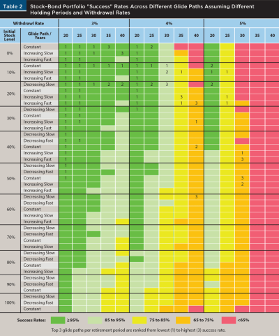
Table 2 shows the success rates of the various glide paths and different initial stock levels (43 different cases) for withdrawal rates of 3, 4, and 5 percent and for retirement periods ranging from 20 to 40 years. A retiree looking at just a 20-year horizon would have a high probability of success with most glide path options, even with a relatively high 5 percent withdrawal rate. However, a typical 67-year-old female retiree has almost a 50 percent chance of living longer than this. If a retiree wants to plan on 30 years of retirement income, there are many cases with a high probability of success with both 3 and 4 percent withdrawal rates, but the picture is not quite as rosy with a 5 percent withdrawal rate. Instead of an 85 percent or better probability of success, the best alternatives at that higher withdrawal rate have probabilities of success ranging from just 65 to 75 percent. The best glide path for the 5 percent withdrawal rate in this case was a 40 percent initial allocation to stock that increases slowly over time. With a 40-year retirement horizon, the 3 percent withdrawal rate still provided many alternatives with a high probability of success. On the other hand, the success of a 5 percent withdrawal rate at this long time horizon was on par with a flip of a coin, or worse, regardless of the glide path followed.

Utility Model

Simple success rates for different starting equity allocations and glide paths for stock–bond portfolios do not provide sufficient information for retirees with other guaranteed sources of income or for those interested in leaving a bequest to their heirs. An investment plan that is “successful” in terms of providing income over the retiree’s life might leave the retiree’s heirs with a terminal value of only $1 or $1 million. If all the retiree is concerned about is lifetime income, that would not matter. However, if leaving a legacy is an important consideration, then the difference is obviously significant. Likewise, “success” from the stock–bond portfolio may be less important if 75 percent of the retiree’s desired income is guaranteed by Social Security and/or other annuities. A failure that leaves someone 25 percent worse off is much less worrisome than one that leaves them with nothing.

To look beyond some of the shortcomings of simple portfolio success rates, a model of constant relative risk aversion (CRRA) is used to examine retiree utility of income (or consumption) under different scenarios. The analysis includes different sets of assumptions related to risk aversion and the desire to leave a bequest. In general, risk averse investors prefer lower, guaranteed income to higher, uncertain income levels. CRRA utility measures have characteristics that are consistent with typical investors/retirees and can be used to model both risk-averse and risk-seeking investors. The basic form of the CRRA function for the utility U of income is shown in equation 5:

(5)

where y is a measure of the investor’s level of risk aversion. While a particular investor’s measure of y is not something that anyone would be expected to know, financial planners do understand the relative level of risk aversion that their clients have. This model is used to measure the expected utility of investors categorized by their degree of risk aversion. Higher levels of y mean the investor is more risk averse, preferring more stable income, even if it is a lower amount. Three different levels of y were used in the analysis to model low, moderate (mid), and high levels of risk aversion.

CRRA measures also exhibit diminishing marginal utility, which means that while utility does increase with more income, it does so at a diminishing rate. For example, suppose there is a retiree with $100,000 in annual income. If they could increase their income to $130,000 per year, they would have a higher utility level, but it would not be 30 percent higher. This also means that the reduction in utility for a given reduction in income is more than the gain in utility for a comparable gain in income, which is one of the central notions of prospect theory (Kahneman and Tversky 1979). So, in this case, the pain that a retiree would feel if their income dropped by $30,000 would be greater than the pleasure they would feel if their income increased by that same $30,000. The degree to which this is true depends on the investor’s level of risk aversion y.

The utility model described briefly below and in more detail in the Appendix was based on the models used by Blanchett (2014) and Blanchett (2015), which considered the percentage of desired income that was replaced in each simulation path. Since the simulations were conducted with nominal cash flows, the percentage of desired income replaced was more relevant than the actual dollar amount of income that was generated. This is because in times of high inflation, higher income would be needed to cover the same basic level of spending power, with no increase in realized utility. Likewise, in times of low inflation, retirees can maintain a constant level of utility with lower levels of income. Scaling based on desired income levels adjusts for inflation and allows for comparisons across different potential economic outcomes. 

A retiree was assumed to begin with a certain income level and a goal of increasing that income each year based on inflation, so that they could maintain constant spending power. That retiree income comes from a combination of Social Security income (SSI_t) and portfolio income (PI_t). Inflation was a random factor in each simulation from period to period, and this directly impacted the amount of income needed to maintain a constant level of utility. Blanchett’s (2014, 2015) income replacement percent (IRP_t) shows the percentage of desired (inflation-adjusted) income that was replaced in each period in the different simulation runs. 

(6)

The numerator of this equation is the actual income received, while the denominator is the “desired” income that is needed to maintain the retiree’s standard of living. The desired income levels are the initial income amounts at t = 0 adjusted for inflation over time. It was assumed that retirees would increase their portfolio withdrawals by the rate of inflation for as long as they can in each simulation path. Since Social Security income is automatically adjusted for inflation each year by the government, the income received SSI_t is always equal to the desired amount. With the stock–bond portfolio, the actual portfolio income generated PI_t may or may not be sufficient to cover the desired portfolio income level, DPI_t. The IRP will always be positive because the Social Security portion of the income stream is guaranteed. This means that the percentage of Social Security payments relative to overall income sets the floor level for the IRP calculation. The time t ranges from 1 to 40, or ages 67 to 106 in the model.

The utility model also recognized that some retirees would like to leave behind a financial legacy. Retirees may have different preferences toward leaving a bequest, so three measures in this regard were included: none, moderate (mid), and high. Since each simulation run generated unique inflation assumptions, the potential bequest payouts were compared to the desired income levels based on realized inflation in the individual simulations. The bequest that would be paid if the retiree died in time t is shown as Bequest_t. This bequest amount was scaled as a percentage of the level of desired overall income to give BP_t: 

(7)

The Appendix shows more detail on the mechanics of the utility model, but equation 8 shows a simplified version of what is being considered:

(8)

      Overall Utility=U(IRP)+pref [U(Bequest)]    

The pref variable signifies the strength of the desire to leave a bequest. U(IRP) and U(Bequest) are the utility of the income received and the bequest left by the retiree, respectively. The best glide path choices were those that maximized the certainty equivalents of the average overall utility of the 1,000 different simulations.

Utility Results

One big question is, “Does including guaranteed Social Security payments (or other guaranteed payments) in the analysis impact the asset allocation and glide path decisions of retirees?” Following up on that, “Do retiree risk aversion levels and desires to leave a bequest affect glide path decisions?” The answers to both these questions are “Yes.” The optimal glide path choices are impacted by the value of Social Security relative to the overall portfolio, the withdrawal rate, the risk aversion level of the retiree, and the retiree’s preference as far as leaving a bequest. These findings are discussed in this section. 

Table 3 presents rankings of the expected utility levels of the 43 different glide path options considered assuming a relatively conservative 3 percent withdrawal rate. The glide path option that provided the highest certainty equivalent of overall utility was ranked 1, while the option that did the worst was ranked 43. The rankings are grouped by the value of Social Security as a percentage of overall wealth at the beginning of retirement. Cases with Social Security as 75, 33, and 17 percent of overall wealth are shown. In each of these cases, the overall utility measure was based on both guaranteed Social Security payments and the income from the retiree’s stock–bond portfolio. Rankings where only the utility of the income from the retiree’s stock–bond portfolio was considered provide a comparison to the situation if Social Security is ignored. Within each of the groups, there are several combinations of risk aversion and bequest preferences. Risk aversion levels (y) are low, moderate (mid), and high. The desire to leave a bequest (pref) is rated as none, moderate (mid), and high.

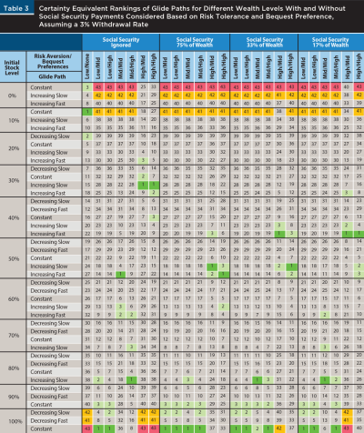
At a 3 percent withdrawal rate, when Social Security was not included in the analysis, investors with a low level of risk aversion and no desire to leave a bequest (low/none) maximized their utility with a 10 percent stock allocation and a constant glide path. All that mattered was providing income over the retiree’s life. However, for the same level of risk aversion, if the desire to leave a bequest was moderate (low/mid) or high (low/high), the preferred glide path choice was a constant allocation of 100 percent stock. The 100 percent stock case was ranked last in the low/none scenario, which was a dramatic shift. Retirees with a low level of risk aversion were the most willing to take extra risk for a higher payoff. In the mid/mid case, 50 percent stock, increasing fast was the top-ranked glide path. The best-case portfolio in the mid/high case was 80 percent stock, increasing slow. The second ranked choice for both mid/mid and mid/high was a 60 percent initial allocation to stock, increasing fast. For retirees with a high level of risk aversion and either a moderate or high desire to leave a bequest (high/mid and high/high, respectively), the same initial allocation of 30 percent stock, increasing slowly over time, was the top portfolio glide path.

The low/none (risk aversion / bequest preference) case where Social Security payments were ignored was the only place where a bequest preference of “none” is presented. This is because with a bequest preference of none, the rankings of the different risk aversion levels showed only minor differences between them. If a retiree places no value on having money left over for heirs, then all that matters is the “success” of the portfolio, which is its ability to provide income over time. With no desire to leave a bequest, utility rankings are primarily impacted by portfolio success over the retirement period. There is no incentive for less risk averse investors to take on higher risk for higher returns because potential payouts are fixed at the inflation-adjusted 3 percent. There were minor differences in the rankings across risk aversion levels, however, because more risk averse investors may place greater weight on distant potential shortfalls. For example, a retiree with a high level of risk aversion was more likely to be concerned with the probability of income shortfalls after age 97, even though they were not likely to live that long, than a retiree with a low level of risk aversion. 

Looking across the grouped wealth categories in Table 3 shows the impact of failing to consider Social Security in the analysis. Compare the scenarios where Social Security was ignored to when Social Security was 33 percent of wealth. The best case for mid/mid shifted from 50 percent stock, increasing fast to 80 percent, increasing slow, respectively. For mid/high, the preferred choice was 80 percent stock, increasing slow, when Social Security was not considered, but it was a constant allocation of 100 percent stock when Social Security was considered. The asset allocation shifts suggested with and without considering Social Security are notable, but not as big, for the high/mid and high/high combinations. Ignoring Social Security, the best glide path for both high/mid and high/high was 30 percent stock, increasing slow. When Social Security was included, the best glide path for both combinations was 40 percent stock, increasing fast.

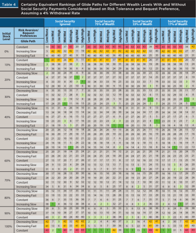
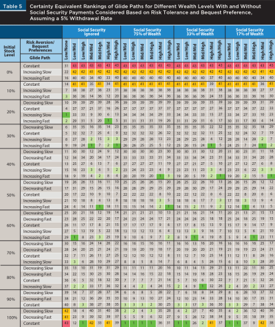
Tables 4 and 5 are organized just like Table 3, except that Table 4 considers utility rankings with a 4 percent withdrawal rate, and Table 5 includes a 5 percent withdrawal rate. Both tables further illustrate the importance of including Social Security payments in the portfolio asset allocation / glide path decision. Consider Table 4, with a 4 percent withdrawal rate and the scenarios where Social Security was ignored versus where Social Security was 33 percent of wealth. The best case for mid/mid shifted from 30 percent stock, increasing fast, to 60 percent stock, increasing fast, respectively. For mid/high, the preferred choice was 50 percent stock, increasing fast, when Social Security was not considered, but a constant 100 percent stock when it was. There were also asset allocation shifts suggested for the high/mid and high/high combinations. Ignoring Social Security, the best glide path for high/high was 20 percent stock, increasing slow. When Social Security was included, the best glide path was 40 percent stock, increasing slow, which was still a sizeable change in portfolio allocations.

Conclusions and Implications for Financial Planners

This paper examined the impact of considering guaranteed Social Security payments in the asset allocation / glide path decision of retirees needing lifetime income. For each starting stock asset allocation level, up to five different glide paths were considered: decreasing slow, decreasing fast, constant, increasing slow, and increasing fast. The impacts of different levels of Social Security relative to overall wealth on portfolio decisions were explored. The paper also took into account varying risk preferences and desires to leave a bequest. 

The results of the paper emphasize the importance of discussions that financial planners have with their clients regarding portfolio risk aversion, factoring Social Security payments into the retirement plan, and how important leaving a bequest is to the client. Despite not having a direct benefit to non-dependent heirs, the level of Social Security retirement payments is a particularly important input in the planning process for retirees who have some desire to leave money behind when they die. When some portion of client financial needs are met with guaranteed income, such as from Social Security, this allows financial planners to focus more of the portfolio on building future wealth for heirs. 

This paper’s findings suggest that most risk-averse retirees who are interested in leaving a bequest should take Social Security payments into account when making their asset allocation decisions. Considering just the stock–bond portfolio in isolation resulted in much lower starting allocations to stock, except for retirees with the lowest level of risk aversion. This was true across all three withdrawal rates that were reported (3, 4, and 5 percent) and for all scenarios involving retirees with moderate (mid) or high risk-aversion levels. Also, the higher the percentage of overall wealth from Social Security (with stocks and bonds making up less), the higher the initial portfolio weights in stock. From one perspective, this makes sense; but from another, it is somewhat counterintuitive. Having a higher proportion of guaranteed income allows the retiree to take on more risk with the stock–bond portion of their wealth, so that makes sense. But there is also another way to look at this. All else equal, lower relative levels of Social Security mean higher values for the stock–bond portfolio, which also means higher overall wealth. General guidance suggests that wealthier individuals should take more risk (more stock), but assuming given withdrawal rates, holding lower stock levels maximizes utility. 

There is a second counterintuitive finding in the paper. For moderate and high risk-averse retirees, most of the top three glide path choices had asset allocations to stock increasing over time. Typical portfolio guidance suggests that stock balances should decline over time, comparable to the “decreasing slow” and “decreasing fast” glide paths in the paper. Blanchett (2015) found a strong preference for declining glide paths; however, that paper had different glide paths and ranked them differently. Blanchett (2015) also noted that the declining glide paths he found could be attributed to the assumption in that paper that interest rates for bonds would start out low and increase over time. Pfau and Kitces (2014) considered portfolio success rates in their analysis, and, like this paper, they found that increasing glide paths were preferable. 

Based on this paper’s findings, financial planners might want to discuss rising glide paths during retirement as an alternative to more traditional declining glide paths with their clients. For example, rather than starting with a 60 percent allocation to stock that declines over time, a retiree could begin with a more conservative 40 percent allocation to stock that they instead increase over time. With a 4 percent withdrawal rate, glide paths of 40 percent stock increasing slow or fast provided higher levels of utility to investors with a high level of risk aversion and a moderate or high desire to leave a bequest than glide paths of 60 percent stock decreasing slow or fast. One of the biggest threats to a portfolio’s success at providing lifetime income is a big loss in value early, rather than later, in retirement. Lower up-front allocations to stock would potentially leave a retiree less susceptible to this sequence risk. The increasing steps upward in the stock allocation would come if the portfolio successfully weathers the early retirement years and the safety cushion of the overall portfolio increases. As the retirement time horizon shortens and the desired income stream from the portfolio becomes more certain, the focus of the portfolio gradually shifts. Instead of focusing on guaranteeing the retiree’s income needs, the portfolio management could emphasize growth for the future heirs, which is where the higher allocations to stock come into play. 

This research comes with a few caveats. While both this paper and Pfau and Kitces (2014) supported rising equity glide paths during retirement, this strategy is not widely accepted. This is an area where more research is still needed. Also, as is true with any long-term financial plan, the preferred glide paths discussed might be the basis for initial retirement road maps, but the course is subject to change as conditions dictate. For example, a big loss in the portfolio early in retirement might dictate changes in withdrawal rates and asset allocations. The planned increases in stock might or might not materialize. That is one of the many reasons that retirees need financial planners.  

Appendix: Income Preference Utility Model

The overall utility model outlined here follows Blanchett (2014) and Blanchett (2015), with one significant change, which is noted below. First, Blanchett’s income replacement percents (IRPs) from equation 5 were calculated for each period. Then, the expected utility of each of the IRPs, U(IRP_t), over time t for all the simulated paths was calculated as:

(A-1)

where y is the level of relative risk aversion. This is the CRRA utility function noted above. While more income is always better in this model, there are diminishing returns as the IRP increases. The level of diminishing returns on utility is dependent on the individual’s level of risk aversion. Three levels of y were assumed for low (0.5), moderate (0.7), and high (0.9) levels of risk aversion.

Each period’s utility measure was adjusted to account for the time value of money and the probability that the retiree would be alive to collect the payment. Since inflation is inherently considered with the actual IRP calculations, real discount rates for each time rr_t were used. Utility for each expected future IRP was discounted to present value terms and adjusted to account for the probability of surviving to collect the payment, Survival_t, giving U(IRP_t)Disc:

(A-2)

The weighted average utility of overall income in each simulation was calculated by: 

(A-3)

where T is the total number of years examined. A 40-year retirement period was considered, which would go to age 107, assuming a retirement age of 67.

The adjusted utility of potential bequest payments was calculated in much the same manner as the utility of Social Security and portfolio income. Starting with the bequest percent BP_t from equation 7, the utility of the potential bequest payments U(Bequest_t), the discounted utility U(Bequest_t)_Disc, and the weighted average utility of the bequest potential of each simulation were calculated as follows:

 (A-4)

 (A-5)

 (A-6)

The only difference in these calculations versus those of the IRP is that bequests are only paid if the retiree is deceased, while the income is only collected if the retiree is alive. The probability of dying in a particular period Deceased_t starts out relatively low and increases over time. Consider the case of a stock–bond portfolio that decreases in inflation-adjusted terms over time due to withdrawals. If the retiree dies early, the heirs would get a higher bequest, but this higher potential payout has a relatively low impact on expected utility because the probability of an early death Deceased_t is low. In this paper, the bequest (as a percent of desired income) was treated the same as the IRP as far as utility goes. The notion of constant relative risk aversion was applied to both the bequest and income. So, for example, while leaving a bequest of $2 million is better than leaving $1 million, it does not provide twice the utility. In their overall benefit analysis, Blanchett (2014, 2015), on the other hand, considered just the raw bequest amount.

Next, the weighted average utility of each simulation was calculated while considering an additional bequest preference factor that recognized that retirees have different desires as far as leaving money to heirs. For some retirees, a bequest may not be a consideration at all. Others may consider leaving money to heirs to be a top priority, and there is room in between these extremes. Bequest preference factors, pref, of 0, 0.5, and 1.0 were included to represent no, moderate (mid), and high desires to leave an inheritance, respectively. 

Finally, the overall certainty equivalent (CE) considering all of the simulations is given by:

 (A-7)

where s represents the individual simulations, and S is the total number of simulations. These certainty equivalents formed the basis of the rankings in Tables 3, 4, and 5.

Citation

Waggle, Doug, and Pankaj Agrrawal. 2024. “Guaranteed Income and Optimal Retirement Glide Paths.” Journal of Financial Planning 37 (6): 74–94.

Endnotes

1. See the Federal Reserve Bank of New York for historical rates: www.newyorkfed.org/markets/reference-rates/effr.
2. Over the period 1/2022 to 12/2023, during which  the Treasury yield curve inverted, long-term U.S. Treasuries returned about –30%, in comparison to about +34% for the S&P 500. This ignited discussions about the relevance of the 60/40 equity–bond allocation for long-term investors. Mozes and Steffens (2021), for example, discuss the 60/40 allocation for pension funds.
3. The minuscule possibility of living past the age of 107 is ignored. A 67-year-old female would only have about a 0.12 percent chance of living to be 107 years old. 
4. Other cases were also examined, but these are reflective of the overall results noted.
5. Blanchett (2015), for example, considered the case of a single 65-year-old female in his analysis. At that time, the full retirement age for Social Security was 65.
6. See the Open Vault Blog by the Federal Reserve of St. Louis: www.stlouisfed.org/open-vault/2019/january/fed-inflation-target-2-percent.
7. See Beckmann, Gern, and Jannsen (2022), for example.

References

Beckmann, Joscha, Klaus-Jürgen Gern, and Nils Jannsen. 2022. “Should They Stay or Should They Go? Negative Interest Rate Policies under Review.” International Economics and Economic Policy 19 (4): 885–912. https://doi.org/10.1007/s10368-022-00547-4.

Bengen, William P. 1994. “Determining Withdrawal Rates Using Historical Data.” Journal of Financial Planning 7 (4): 171.

Blanchett, David M. 2007. “Dynamic Allocation Strategies for Distribution Portfolios: Determining the Optimal Distribution Glide Path.” Journal of Financial Planning 20 (12): 68–70, 72–81.

Blanchett, David M. 2014. “Determining the Optimal Fixed Annuity for Retirees: Immediate versus Deferred.” Journal of Financial Planning 27 (8): 36–44.

Blanchett, David M. 2015. “Revisiting the Optimal Distribution Glide Path.” Journal of Financial Planning 28 (2): 52–61.

Blanchett, David M. 2017. “The Impact of Guaranteed Income and Dynamic Withdrawals on Safe Initial Withdrawal Rates.” Journal of Financial Planning 30 (4): 42–52.

Blanchett, David M., and Michael Finke. 2018. “Annuitized Income and Optimal Equity Allocation.” Journal of Financial Planning 31 (11): 48–55.

Blanchett, David M., Michael Finke, and Wade D. Pfau. 2013. “Low Bond Yields and Safe Portfolio Withdrawal Rates.” The Journal of Wealth Management 16 (2): 55–62,7.

Cooley, Philip L., Carl M. Hubbard, and Daniel T. Walz. 2011. “Portfolio Success Rates: Where to Draw the Line.” Journal of Financial Planning 24 (4): 48–50, 52–54, 56–60.

Cox, John C., Jonathan E. Ingersoll, and Stephen A. Ross. 1985. “A Theory of the Term Structure of Interest Rates.” Econometrica (Pre-1986) 53 (2): 385–407.

Finke, Michael, Wade D. Pfau, and David M. Blanchett. 2013. “The 4 Percent Rule Is Not Safe in a Low-Yield World.” Journal of Financial Planning 26 (6): 46–55.

Finke, Michael, Wade D. Pfau, and Duncan Williams. 2012. “Spending Flexibility and Safe Withdrawal Rates.” Journal of Financial Planning 25 (3): 44–51.

Kahneman, Daniel, and Amos Tversky. 1979. “Prospect Theory: An Analysis of Decision Under Risk.” Econometrica (Pre-1986) 47 (2): 263–91.

Kitces, Michael E., and Wade D. Pfau. 2015. “Retirement Risk, Rising Equity Glide Paths, and Valuation-Based Asset Allocation.” Journal of Financial Planning 28 (3): 38–48.

Mozes, Haim A., and John Launny Steffens. 2021. “The Outlook for Endowment and Pension Funds.” The Journal of Wealth Management 24 (1): 120–31. https://doi.org/10.3905/jwm.2021.1.131.

Pfau, Wade D. 2011. “Can We Predict the Sustainable Withdrawal Rate for New Retirees?” Journal of Financial Planning 24 (8): 40–47.

Pfau, Wade D., and Michael E. Kitces. 2014. “Reducing Retirement Risk with a Rising Equity Glide Path.” Journal of Financial Planning 27 (1): 38–45.

Spitzer, John J., and Sandeep Singh. 2008. “Shortfall Risk of Target-Date Funds during Retirement.” Financial Services Review 17 (2): 143–53.

Waggle, Doug, Gisung Moon, and Hongbok Lee. 2022. “Retirement Glide Path Options in an Uncertain, Low-Interest-Rate Environment.” Journal of Financial Planning 35 (3): 68–88.