Journal of Financial Planning: January 2014
Wade D. Pfau, Ph.D., CFA, is a professor of retirement income at The American College and the 2011 recipient of the Journal’s Montgomery-Warschauer Award. He hosts the Retirement Researcher blog at wpfau.blogspot.com. Send an email to Wade Pfau.
Michael E. Kitces, CFP®, CLU®, ChFC®, RHU, REBC, is a partner and the director of research for Pinnacle Advisory Group and the publisher of The Kitces Report newsletter and the financial planning industry blog Nerd’s Eye View through his website www.kitces.com. Send an email to Michael Kitces.
Executive Summary
- This study explores the issue of what is an appropriate default equity glide path for client portfolios during the retirement phase of the lifecycle.
- Results show, surprisingly, that rising equity glide paths in retirement—where the portfolio starts out conservative and becomes more aggressive through the retirement time horizon—have the potential to actually reduce both the probability of failure and the magnitude of failure for client portfolios.
- Overall, the results show that rising equity glide paths from conservative starting points can achieve superior results, even with lower average lifetime equity exposure. For instance, a portfolio that starts at 30 percent in equities and finishes at 60 percent performs better than a portfolio that starts and finishes at 60 percent equities. A steady or rising glide path provides superior results compared to starting at 60 percent equities and declining to 30 percent over time.
Conventional wisdom suggests an “age in bonds” style asset allocation strategy over a person’s lifetime. During the accumulation phase, this can be justified theoretically by considering a household’s entire balance sheet including human capital. When young, most clients have saved little. Their main asset will be the present value of lifetime future earnings, which gives them the capacity to take significant risks with their financial capital. As their time horizon to retirement shortens and the buffer value of their human capital declines, so too does their capacity for financial risk. Their equity exposure should decline accordingly.
At retirement, human capital falls to zero. However, because of the need to provide for an extended period of retirement income and generate growth necessary to maintain inflation-adjusted withdrawals, equity exposure typically does not fall all the way to zero. Nonetheless, even with some equity exposure at the start of retirement, many advisers still justify the concept of a declining equity exposure throughout retirement on the basis that a retiree’s time horizon shortens with each passing year. Arguably, for someone willing to pay careful attention to the evolving funding status of their retirement (the present value of their remaining assets divided by the present value of their remaining liabilities), asset allocation can be adjusted dynamically by matching assets to liabilities in coordination with the client’s risk capacity and risk aversion, rather than just on an arbitrary path.
For those unwilling to take such care, including users of target date or lifecycle asset allocation funds, or for those whose goals are somewhat more complex in the balancing of current and future income and legacy goals, what should be the default equity glide path in the postretirement period?
The purpose of this study is to address this question. Results suggest that rising equity glide paths in retirement have the potential to reduce both the probability and magnitude of failure for client portfolios. Just as equity exposure can be more beneficial for those who are very young, so too can greater equity exposure in the later years of retirement actually help, especially in those scenarios where returns in the early retirement years are poor. In essence, the optimal equity exposure for a portfolio over an accumulation/decumulation lifetime may look less like a slow and steady downward slope, and more like the letter U, in which the stock allocation is the lowest at the point when lifestyle spending goals are most vulnerable to absolute losses in wealth (the retirement transition itself), but greater in both the earliest years and also the latest.
Literature Review
There is a deep body of literature studying what retirees may treat as a sustainable withdrawal rate from a portfolio of volatile assets over a long retirement period. Pfau (2012a) provided an overview of this literature, dividing studies between those based on examining rolling periods from U.S. historical data, Monte Carlo simulations with parameters chosen based on the historical data, and Monte Carlo simulations with parameters defined differently from the U.S. historical record. Kitces (2012) also provided an overview of the research on these questions extending back to Bengen (1994). He addressed how the initial studies have been modified to consider factors such as taxes, expenses, time horizons, deeper asset class diversification, variable spending, risk tolerance, market valuations, partial annuitization, and desires to leave a legacy.
This paper extends the literature by focusing on studies of sustainable withdrawal rates in retirement in which asset allocations are not fixed. The earliest study about the impact of asset allocation glide paths on retirement sustainability is Bengen (1996), who focused on the comparison between fixed asset allocations and declining equity glide paths. In particular, he compared maintaining a fixed 63 percent stock allocation over retirement to strategies with various annual reductions to the stock allocation over a 30-year period. He found that the SAFEMAX (the highest sustainable withdrawal rate in the worst-case scenario from history) became smaller as the pace of the stock phasedown increased (that is, sustainable withdrawals were lower when equity exposure declined through retirement). Bengen also found that with rolling historical simulations, a phasedown in the stock allocation helped protect the remaining portfolio value. With modest declining glide paths, the SAFEMAX impact was modest. He concluded that a 1 percent annual phasedown in the stock allocation was an appropriate compromise between growing wealth, supporting the withdrawal rate, and reducing late retirement volatility.
Subsequently, Blanchett (2007) used Monte Carlo simulations to test fixed asset allocations against a wide variety of glide paths that reduce the equity allocation during retirement. Using numerous outcome metrics, Blanchett concluded that fixed asset allocations provided superior results compared to approaches that reduce allocation to equities later in retirement.
The literature indicates three potential reasons to vary the asset allocation over retirement. The first is a valuation-based approach in which asset allocation is adjusted to stock market valuation levels (Kitces 2009; Pfau 2012b). A second approach is to consider asset liability matching, in which assets are linked to specific goals. Huxley and Burns (2005) exemplified this approach from a more probability-based outcome perspective, while Branning and Grubbs (2010) justified the idea from a safety-first perspective by using secure assets to meet essential needs. Those using these approaches do not set an asset allocation in advance. Asset allocation results from the process of asset-liability management.
A related approach is the adaptive model (Fan, Murray, and Pittman 2013). This approach considers a client’s spending needs and uses equity exposure as a lever to manage shortfall risk. Typically, this model indicates that beginning retirement with a lower equity allocation reduces the sequence of returns risk, with the equity allocation becoming more aggressive later in retirement when the client enjoys at least satisfactory market performance.
The third approach (and the one most closely linked to this study) is based on general tests of glide paths separated from individual specific spending goals rather than looking to find what is feasible and how to obtain the largest sustainable withdrawals from a portfolio. Cohen, Gardner, and Fan (2010) found evidence in support of a rising equity glide path after retirement. They considered whether target date funds should be managed “to” or “through” retirement, and then considered more carefully that the post-retirement period may present different implications for investors. Spitzer and Singh (2007) determined that rebalancing the asset allocation for a retirement income portfolio is not important, and that a strategy of spending bonds first does not increase shortfall risk. Although not specifically articulated, their findings imply a beneficial impact for a rising equity glide path. Kitces and Pfau (2013) examined glide path effects in the context of understanding the different ways that partial annuitization impacts a retirement income portfolio. They found that some of the implied benefits of partial annuitization can be attributed to the rising equity glide path the strategy creates when viewed from a household balance sheet perspective.
Methodology
This research investigates the sustainability of constant inflation-adjusted spending strategies from a portfolio of financial assets. The hypothetical retirees described in this study are attempting to finance a particular spending goal, which is an inflation-adjusted amount equal to either 4 percent or 5 percent of initial retirement date assets, and to sustain that income stream for a set number of retirement years. The baseline results presented here are for retirements of 30 years, but 20- and 40-year scenarios also will be discussed.
The analysis was premised on the maximum sustainable withdrawal rate (MWR). As defined here, MWR is the highest withdrawal rate that would have provided a sustained real income over a given retirement duration. At the beginning of the first year of retirement, an initial withdrawal is made equal to the specified withdrawal rate multiplied by the accumulated wealth. Remaining assets then grow or shrink according to the asset returns for the year. At the end of the year, the remaining portfolio wealth is rebalanced to the targeted asset allocation. In subsequent years, the withdrawal dollar amount adjusts by the previous year’s inflation rate and the order of portfolio transactions is repeated. Withdrawals are made at the start of each year and the amounts are not affected by asset returns, so the current withdrawal rate (the withdrawal amount divided by remaining wealth) differs from the initial withdrawal rate in subsequent years. If the withdrawal pushes the account balance to zero, the withdrawal rate was too high and the portfolio failed. The MWR is the highest rate that succeeds. Taxes are not specifically incorporated, and any taxes associated with the entire portfolio would still need to be paid.
Within this context, four outcome measures were investigated. First was the failure rate, which is the probability of financial asset depletion over different time horizons (20, 30, or 40 years) for those using either a 4 percent or 5 percent initial withdrawal rate with subsequent inflation adjustments to those amounts.
Second, we focused on the potential magnitude of failure. Magnitude of failure was evaluated by measuring the amount of financial assets remaining in the 5th percentile of the distribution of outcomes when using a 4 percent or 5 percent withdrawal rate. If the failure rate for the strategy was greater than 5 percent, then remaining financial assets would be negative, indicating a shortfall below the client’s lifetime spending goal. In this case, the shortfall was calculated as the sum of inflation-adjusted spending needs in today’s dollars that could not be satisfied over the retirement period, without any further discounting of these values. If the failure rate was less than 5 percent, then there would be a surplus of wealth at the 5th percentile of the distribution.
The shortfall or surplus shown in the tables is based on total retirement date wealth of 100. Given annual spending amounts of 4 percent or 5 percent of real starting wealth, a shortfall of –12 with a 4 percent withdrawal rate means the retiree ran out of financial assets with three years left in the retirement period; alternatively, a legacy of +16 would indicate there was four years’ worth of spending still remaining (subject to the impact of subsequent market returns), even in the 5th percentile outcome. This measurement provides an indication of the magnitude of failure. A larger spending shortfall implies that financial assets were depleted sooner in the retirement period.
Third, the analysis reflects on the upside potential of the strategy. This measure is the real amount (in today’s dollars) of financial assets remaining at the end of the retirement period in the median outcome of the Monte Carlo simulations.
Finally, information about the maximum sustainable withdrawal rate supported at the 10th percentile of outcomes is provided. This measure indicates that in 10 percent of cases, the sustainable withdrawal rate was even less, but in 90 percent of cases, sustainable retirement income would have been higher (and/or taking withdrawals at a lower rate would result in a greater final legacy).
These outcome measures were calculated from 10,000 Monte Carlo simulations for 121 lifetime asset allocation glide paths. At retirement, the initial stock allocation ranges from between zero and 100 percent in 10 percentage point increments (11 possibilities). The asset allocation in the final year of retirement also ranges between zero and 100 percent in 10 percentage point increments. In the intervening years of the retirement, the asset allocation of the glide path adjusts annually in a straight line between the initial and final asset allocation.
For example, consider a 30-year retirement with an initial stock allocation of 30 percent and a final stock allocation of 60 percent. In each year of retirement, the portfolio rebalances to a stock allocation that rises by 1 percent per year over the 30 years. After 10 years, the stock allocation is 40 percent. After 25 years, the stock allocation is 55 percent, and by year 30, the allocation is 60 percent. This approach allows for fixed glide paths, declining equity glide paths, and rising equity glide paths of varying degrees, depending on the starting and end points, the magnitude of the difference between them, and the number of years to execute the glide path itself.
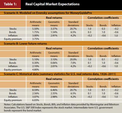
Table 1 shows the real return capital market expectations used to guide the 10,000 Monte Carlo simulations. For the baseline, we used the real return assumptions prepared by Harold Evensky for the MoneyGuidePro software as of July 2013. To understand more about the implications for different capital market assumptions, we also considered a second scenario more closely calibrated to the low interest rate environment affecting today’s retirees and a third scenario with stock and bond returns based on the more optimistic historical real return averages found in Ibbotson’s Stocks, Bonds, Bills, and Inflation yearbook. Simulations were made in each case with a multivariate lognormal distribution defined by these parameters. In essence, the scenarios varied assumptions for real bond returns, real stock returns, and/or the equity risk premium.
Results
Across all time horizons and withdrawal rates, when examining the approach that provides the highest sustainable withdrawal rates given a prospective 10 percent failure rate, the results consistently show support for rising equity glide path portfolios.
Declining equity glide paths do not necessarily help support retirement success. Static allocations generally fare worse than more conservative starting allocations that rise in equity exposure throughout retirement. Depending on the underlying assumptions, the optimal starting equity exposures are generally around 20 percent to 40 percent and finish at around 40 percent to 80 percent. With the Evensky return assumptions used as a baseline in this study, the optimal end point of the glide path was generally less than with historical return assumptions, as the equity risk premium is less. This reduces the return-enhancing benefits of equities. Nonetheless, some degree of a rising glide path is still supported with all three sets of capital market assumptions.
When modeled relative to the success of a 4 percent or 5 percent withdrawal rate, the results varied depending on the details of the return assumptions and the target spending level. For example, Table 2 shows the success rates at a 4 percent withdrawal rate using the Evensky assumptions for various glide paths. These figures demonstrate that rising equity glide paths generally fared best by a small margin. The highest success rate on the chart, signified by the standalone box around the result, shows that an initial allocation of only 30 percent in equities at retirement, rising to 80 percent by the end of retirement, provides the highest success. More generally, any allocations that begin at 20 percent to 40 percent in equities and finish at 60 percent to 80 percent provide the highest success rates. This is notable given that these approaches have less equity exposure during the years when the portfolio size effect is greatest. These outcomes are typically superior to static asset allocations that simply maintain the same average equity exposure throughout retirement.
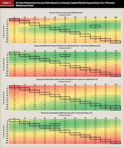
Results reveal that rising glide paths are even more effective when examined from the perspective of the potential shortfall at the 5th percentile, especially when the glide path starts off conservatively. The most favorable shortfall actually occurs with a glide path that starts at only 10 percent in equities and rises to 50 percent in equities. When viewing the maximal withdrawal rate at the 10th percentile a similar result occurs, with the optimal portfolio starting at 20 percent in equities and ending at 40 percent. Notably, portfolios that start off in the 10 percent to 30 percent equity range and use rising glide paths fare far better than static portfolios with 50 percent or 60 percent in equities. Rising glide paths also result in better outcomes when compared to portfolios that use a declining glide path.
From the perspective of traditional retirement planning projections, these results may seem surprising. The third panel of Table 2 reveals why: when viewed from the perspective of the median amount of wealth at the end of the period, results improve as equity exposures increase, given that, on average, higher equity exposures result in greater average returns. In other words, when viewing the median results, greater equity exposures are more appealing. It is only when examined from the perspective of risk and magnitude of shortfalls that the optimal portfolios not only contain far less equity exposure on average, but also perform best when the equity exposure starts very low and rises throughout retirement.
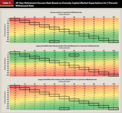
When tested at higher withdrawal rates, where the risk of failure is elevated, especially using Evensky assumptions as shown in Table 3, results reveal that retirees fare best with the greatest equity risk at the beginning of retirement, as the top-performing scenarios begin with at least 80 percent in equities. This is not entirely surprising. If the withdrawal rate places enough pressure on the portfolio’s potential growth rate, at some point taking significant risks in equities and just hoping for favorable outcomes is the best path to maximize the likelihood of success. From the perspective of viewing the magnitude of potential shortfalls, however, the optimal portfolio remains a rising equity glide path (starting at 10 percent in equities and finishing at 60 percent). This finding is similar to the 4 percent withdrawal rates at the same returns.
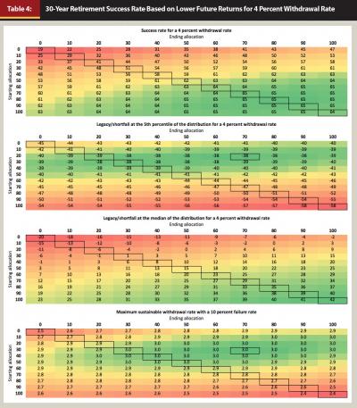
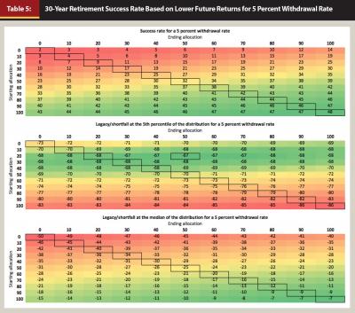
Investigating the lower return environment in Tables 4 and 5, which assumes that fixed income returns sustain at today’s ultra-low levels but that the historical equity risk premium remains intact, creates a more noticeable distinction. When simply trying to maximize the probability of success, retirees are compelled to take significant equity risk. The best portfolios start and finish at significant equity exposures. However, for those trying to manage potential retirement shortfalls, controlling for material risk exposure, more conservative rising equity glide paths fare better by minimizing the magnitude of shortfalls even while increasing the likelihood.
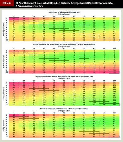
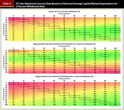
Tables 6 and 7 show the results of the glide paths using long-term historical returns. In this scenario, with both higher overall returns and a greater equity risk premium, rising equity glide paths perform even better. The results are more consistent in showing an optimal retirement glide path that begins at 30 percent equities and rises to 70 percent equities by the end in terms of probability and magnitude of failure. In the higher return environment, these portfolios fare noticeably better than 60/40 static portfolios and materially better than just keeping the portfolio invested conservatively. At a 5 percent withdrawal rate, the results are generally the same, although the greater pressure on withdrawals increases the benefit of starting (and finishing) with slightly more in equities overall to have a reasonable chance of generating the requisite returns.
The analysis also considered time horizons of 20 years. The results hold as well. Rising equity glide paths that start around 20 percent in equities and finish at 50 percent to 70 percent in equities are generally optimal, as long as there is still a reasonable equity risk premium. Using the return assumptions as described earlier with a compressed equity risk premium, the optimal results start with almost no equities and only increase exposure to about 30 percent by the end. Given the shorter time horizon, there simply is not much time for equities to provide a benefit in light of their volatility.
With longer time horizons (40 years), the results are again consistent. In situations where the combination of returns and withdrawal rates stresses the portfolio, the optimal results to minimize the risk of failure have fairly significant equity exposure. The approach to minimize the magnitude of failure still involves a rising equity glide path. When the equity risk premium is reduced, the starting equity exposure of the glide path is lower; however, the rising equity glide path is still superior as a way to manage potential shortfalls. These results also hold when tested with lower initial withdrawal rates (3 percent), although the glide path does not need to rise as high when withdrawal rates are more conservative (for example, starting at 10 percent and finishing at 40 percent).
Implications for Financial Planners
The implications of this research for financial planners are significant. Results suggest that the traditional approach of maintaining constant asset allocations in retirement, which are routinely rebalanced, are actually far less than optimal. Although such an approach is actually superior to decreasing equity exposure through retirement, the results of this study reveal that the best solution may be to steadily increase equity exposure throughout retirement, while starting at a lower initial equity exposure.
This result may appear counterintuitive. The traditional argument is that equity exposure should decrease throughout retirement as a retiree’s time horizon and life expectancy shrinks and mortality looms. The problem with this perspective is that it does not account for what causes a client’s retirement to “fail” in the first place. The success of a retirement scenario is heavily influenced by the sequence of returns. As Kitces (2008) showed, in the case of a 30-year time horizon, the outcome of a withdrawal scenario is dictated almost entirely by the real returns of the portfolio for the first 15 years. If the returns are good, the retiree is so far ahead relative to the original goal that a subsequent bear market in the second half of retirement has little impact. Although it is true that final wealth may be highly volatile in the end, the initial spending goal will not be threatened. By contrast, if the returns are bad in the first half of retirement, the portfolio is so stressed that the good returns that follow are absolutely crucial to carry the portfolio through to the end.
In this context, the problem with declining equity glide paths becomes clear. In scenarios that threaten retirement sustainability, such as an extended period of poor returns in the first half of retirement, a declining equity exposure over time will lead the retiree to have the least in stocks when the good returns finally show up in the second half of retirement. This is also why rising equity glide paths perform better—in a situation where the first half of retirement is bad, rising equity exposure leads the retiree to systematically dollar cost average into equities through flat or declining markets, maximizing exposure by the time the good returns show up. This helps sustain greater retirement income over the entire time period.
In other words, in the scenarios where equity returns are bad early on, rising equity glide paths are crucial. In scenarios where equity returns are good early on, the retiree is so far ahead it doesn’t matter (relative to achieving the original goal). Rising equity glide paths create a “heads you win, tails you don’t lose” outcome in securing a starting goal. Of course, retirees who are far ahead may choose to decrease their equity exposure later simply because they have a significant amount of newfound wealth, but the point remains that they do not need to reduce their equity exposure to secure their goals if they’re that far ahead in the first place.
Accordingly, for those households looking to maximize their level of sustainable retirement income, and/or to reduce the potential magnitude of any shortfalls in adverse scenarios, portfolios that start off in the vicinity of 20 percent to 40 percent in equities and rise to the level of 60 percent to 80 percent in equities generally perform better than static rebalanced portfolios or declining equity glide paths. The results hold even in situations where the final equity exposure is no higher than what the client’s static portfolio allocation may have been in the first place.
The results also reveal that in particular scenarios where the equity risk premium is depressed, the optimal glide path includes less equity overall. In scenarios where the goal is to withdraw at a level that stresses the portfolio and its expected growth rate, higher overall levels of equity are necessary (with such high-risk goals, having a relatively high-risk portfolio, even with the danger this approach entails, is still the optimal solution).
In general, for those who are looking to maximize a sustainable income level, or determine the amount of assets to support a (reasonable) target income level, rising equity glide paths appear to maximize the likelihood of success and sustainable income, and reduce the magnitude of shortfalls when they occur.
The clear caveat of this approach is that it may create concerns for seniors in their later years. Seniors may not be comfortable, from a risk tolerance perspective, handling the greater equity exposures implied by this approach. On the other hand, in many scenarios, the optimal rising equity glide paths still finish with little more in equities than the 60/40 portfolios that are commonly used by many planners anyway; thus, the approach actually results in less average equity exposure throughout retirement, less portfolio volatility along the way, and a portfolio that finishes with no more equity exposure than a static approach would have implied.
Planners may be able to find ways to frame rising equity glide path strategies in a manner that is more comfortable for clients. For instance, a “bucket strategy” that draws heavily from the fixed income allocation in the early years and allows equities to grow is effectively a rising glide path strategy. Kitces and Pfau (2013) showed that partial annuitization strategies also essentially represent a form of a bucketing-based rising equity glide path approach.
Ultimately, most financial planners will still craft customized, individualized recommendations for their clients and not necessarily use glide paths (rising or otherwise); furthermore, most planners will still be monitoring a client’s progress on an ongoing basis, making adjustments as necessary rather than based upon a static formula. Nonetheless, the results of this study are significant, as the findings imply that the default glide path should be to start with a much lower equity exposure than is traditionally used and increase it over time. Further actions from the planner and client should be intentional efforts to deviate from this default position.
References
Bengen, William P. 1994. “Determining Withdrawal Rates Using Historical Data.” Journal of Financial Planning 7 (4): 171–180.
Bengen, William P. 1996. “Asset Allocation for a Lifetime.” Journal of Financial Planning 9 (8): 58–67.
Blanchett, David M. 2007. “Dynamic Allocation Strategies for Distribution Portfolios: Determining the Optimal Distribution Glide Path.” Journal of Financial Planning 20 (12): 68–81.
Branning, Jason, and M. Ray Grubbs. 2010. “Using a Hierarchy of Funds to Reach Client Goals.” Journal of Financial Planning 23 (12): 31–33.
Cohen, Joshua R., Grant W. Gardner, and Yuan-An Fan. 2010. “The Date Debate: Should Target Date Fund Glide Paths Be Managed ‘To’ or ‘Through’ Retirement?” Russell Investments Research Report.
Fan, Yuan-An, Steve Murray, and Sam Pittman. 2013. “Optimizing Retirement Income: An Adaptive Approach Based on Assets and Liabilities.” Journal of Retirement 1 (1): 124–135.
Huxley, Stephen J., and J. Brent Burns. 2005. Asset Dedication: How to Grow Wealthy with the Next Generation of Asset Allocation. New York: McGraw-Hill.
Kitces, Michael E. 2008. “Resolving the Paradox: Is the Safe Withdrawal Rate Sometimes Too Safe?” The Kitces Report (May).
Kitces, Michael E. 2009. “Dynamic Asset Allocation and Safe Withdrawal Rates.” The Kitces Report (April).
Kitces, Michael E. 2012. “Practical Applications of 20 Years of Safe Withdrawal Rate Research.” The Kitces Report (March).
Kitces, Michael E., and Wade D. Pfau. 2013 (in press). “The True Impact of Annuities on Retirement Sustainability: A Total Wealth Perspective.” Retirement Management Journal.
Pfau, Wade D. 2012a. “Capital Market Expectations, Asset Allocation, and Safe Withdrawal Rates.” Journal of Financial Planning 25 (1): 36–43.
Pfau, Wade D. 2012b. “Withdrawal Rates, Savings Rates, and Valuation-Based Asset Allocation.” Journal of Financial Planning 25 (4): 34–40.
Spitzer, John J., and Sandeep Singh. 2007. “Is Rebalancing a Portfolio During Retirement Necessary?” Journal of Financial Planning 20 (6): 46–57.
Citation
Pfau, Wade D., and Michael E. Kitces. “Reducing Retirement Risk with a Rising Equity Glide Path.” Journal of Financial Planning 27 (1): 38–45.