Journal of Financial Planning: August 2014
David Blanchett, CFP®, CFA, is head of retirement research at Morningstar Investment Management. Email author HERE.
Acknowledgments: The author thanks Michael Kitces and Wade Pfau for helpful comments and edits.
Executive Summary
- This paper contrasts the relative efficiency of single premium immediate annuities (SPIAs) and deferred income annuities (DIAs) for a variety of retirement scenarios. The analysis considers not only traditional nominal SPIAs and DIAs, but also includes variations with inflation riders and period certain benefits.
- Based on the analysis, the optimal form of guaranteed income varies materially depending on model assumptions and retiree preferences. Nominal SPIAs, especially those with a 20-year certain payment period, tend to be the most efficient among the eight annuity types considered in this analysis, on average, followed by nominal SPIAs and nominal DIAs. However, if DIA payout rates increase by only 5 percent, nominal DIAs become the most attractive option, on average.
- Although DIAs may be slightly less efficient than SPIAs today, on average, that gap will likely close as the DIA market place becomes more competitive.
- Results suggest DIAs appear to offer significant promise to retirees as an efficient form of guaranteed income, especially given the relatively low cost for the longevity hedge when compared to SPIAs.
Please click HERE to access Appendices 1-3 (referenced within the article).
Deferred income annuities (DIAs), also commonly referred to as longevity insurance, have recently received significant attention in the media and from retirees and financial planners. DIAs provide guaranteed income for life, but unlike single premium immediate annuities (SPIAs), the benefit payments for DIAs do not begin until some future point in time (versus immediately for SPIAs). For example, a retiree could purchase a DIA at age 65 where benefits commence at age 85. If the annuitant does not live until age 85, no benefits will be received (in the absence of some type of minimum benefit rider); however, after turning 85, benefits will then be guaranteed for life (or potentially a period certain depending on the type of DIA purchased).
In theory, DIAs offer a more efficient hedge against longevity risk than SPIAs, because the effective cost of the insurance is lower. This is because only those individuals who survive to the benefit commencement age will receive any benefit payments, and even those who do receive payments may not do so for long. This paper tests this premise and explores the relative efficiency of SPIAs and DIAs for a variety of retirement scenarios. The analysis considers not only traditional nominal SPIAs and DIAs, but also includes variations with inflation riders and period certain benefits.
The optimal annuity type was determined using a preference model based on utility. Eight sets of assumptions were varied for the analysis: (1) initial withdrawal rate, (2) equity allocation, (3) percentage of total retirement income need covered by Social Security, (4) nominal returns, (5) inflation, (6) life expectancy, (7) shortfall risk aversion, and (8) bequest preference. For each assumption or preference, three possible values were used: low, moderate, or high. Combined, this resulted in a total of 6,561 scenarios. The approach can lead to conclusions that are more robust than an analysis based on a restricted set of assumptions or scenarios. An autoregressive return model was used for the analysis that explicitly incorporates today’s low bond yields, where yields were assumed to randomly “drift” back toward some higher value over time.
Based on the analysis, the optimal form of guaranteed income (annuity) varies materially depending on the model assumptions and retiree preferences; however, nominal SPIAs, especially those with a 20-year certain payment period, tend to be the most efficient, on average, followed by nominal SPIAs and nominal DIAs. If DIA payout rates increase by 5 percent, though, DIAs become the most attractive option, on average. Therefore, although DIAs may be slightly less efficient than SPIAs today, on average, that gap is likely to close as the DIA market place becomes more competitive. In summary, DIAs appear to offer significant promise to retirees as an efficient form of guaranteed income, especially given the relatively low cost for the longevity hedge when compared to SPIAs.
SPIAs and DIAs
DIAs are a fairly recent innovation, coming to market over the last five years or so. Milevsky (2005) was one of the first to note the potential benefit of DIAs, which he referred to as an advanced-life delayed annuity (ALDA). Milevsky’s ALDA included inflation protection, where benefits would only commence at some future advanced age. This is in contrast to SPIAs, which provide income immediately.
DIAs, in theory, represent a more efficient means of transferring longevity risk than SPIAs, because these annuities only provide an income if the annuitant lives to a certain age. This reduces the cost of the insurance, because a good portion of individuals will not survive to the benefit commencement date, and even for those who do, the benefit payments may only last a couple of years. For example, if an individual purchases a DIA (or ALDA) at age 65 where benefits commence at age 85, the probability of that individual receiving a single benefit payment are only approximately 50 percent, because the life expectancy for a 65-year-old is approximately 20 years.
Scott, Watson, and Hu (2007) and Scott (2008) contended that if a household is only prepared to annuitize part of their wealth, it is best to do so for very advanced ages, because the probability of survival is the lowest. Gong and Web (2010) noted that one potential advantage of DIAs over a non-annuitized strategy is that DIAs transform the complex task of decumulating one’s wealth over an uncertain lifespan into the much simpler task of decumulating over a fixed period ending on the date that the DIA payments commence. Therefore, DIAs can provide not only a hedge against longevity risk, but also help simplify the income-generation process during retirement, especially for older ages.
Pfau (2013) conducted a study that is similar in spirit to this analysis, where the optimal amount of assets used to purchase a DIA for various levels of spending shortfalls and real financial assets at death was explored (this concept is similar to shortfall risk and residual wealth concepts). Pfau concluded that relative to a SPIA, a DIA results in better retiree outcomes with more liquidity and the same longevity protection at less cost. This study reaches similar conclusions.
Annuity Features
- Annuity quotes were obtained from CANNEX USA on January 26, 2014 (with an assumed retiree birthday of January 26, 1949). Each quote represents a married couple, male and female, both age 65, with Illinois listed as the state of residence for a non-qualified fund type with annual payments. Four different flavors of each of the two annuity types (SPIAs and DIAs) were considered, based on different potential combinations of either nominal or real benefit payments and whether or not some type of minimum guaranteed benefit exists. This created a total of eight distinct annuity quotes (or annuity types) considered for the analysis. Each annuity includes a 100 percent survivor benefit, so benefit payments will continue in full until both retirees have passed away. The eight annuity types selected, and the attributes of each, are noted below.
Nominal SPIA, life only (5.795 percent payout rate from ING USA Annuity and Life Insurance Co.) - Nominal SPIA, with 20-year term certain (5.712 percent payout rate from ING USA Annuity and Life Insurance Co.)
- Real SPIA, life only (3.885 percent payout rate, payments increase with changes in CPI-U from Principal Group)
- Real SPIA, with 20-year term certain (3.813 percent payout rate, payments increase with changes in CPI-U from Principal Group)
- Nominal DIA, life only (34.806 percent payout rate, benefits commence at age 85, from New York Life)
- Nominal DIA, with cash refund (31.670 percent payout rate, benefits commence at age 85, from New York Life)
- Real DIA, life only (25.451 percent payout rate, benefits commence at age 85, from American General Life Insurance Co.)
- Real DIA, with cash refund (22.730 percent payout rate, benefits commence at age 85, from American General Life Insurance Co.).
The payout rate defines the amount of income received from the annuity type, given the initial purchase amount. For example, the payout rate of 5.795 percent for the nominal SPIA would result in an immediate annual income of $5,795 for an initial purchase of $100,000. For the DIA, the payout rate is the amount of income that will be received at the age of benefit commencement (85) so long as either member of the couple is still living. The potential inflation adjustment to benefits would only take effect after the benefits commence for the DIA. These are assumed to increase annually with inflation.
Not surprisingly, including a benefit inflation adjustment rider and/or a guaranteed payment period rider decreases the payout rate. However, these riders may still have value to some retirees, depending on the retiree’s preferences and the assumptions used for the analysis. For example, a retiree who is concerned about passing away early in retirement may value benefit period certain, even if it reduces the lifetime income.
Although the analysis is based on a joint couple, the results should generally be expected to apply to a single retiree (male or female) as well. This is because annuity payout rates are adjusted accordingly based on mortality expectations. Also, although this analysis focuses on a single delay period for DIAs (20 years, from age 65 to age 85), in reality there are delays of varying periods that may work better for some retirees. This analysis also assumes a retiree can select only one of the eight different annuity types. In practice, some combination among the eight annuity types, or considering an annuity type not considered for this analysis, may be most appropriate.
Return Simulation Model
The majority of research on sustainable withdrawal strategies has used either historical rolling time periods or a stochastic (Monte Carlo) simulation process for returns. Monte Carlo simulations are the most common. The returns for Monte Carlo simulations are typically based on either long-term historical averages or forecasts where the expected return of an asset class is the same for each year of the simulation (although the actual return for a given year of a given run would vary stochastically). These approaches are less useful when there is a significant and sustained deviation, such as the current low bond yield market. The implications of low bond yields on retirement portfolios have been explored previously in a variety of papers by Blanchett, Finke, and Pfau (2013, 2014).
This paper uses an autoregressive return simulation model similar to Blanchett et al. (2013, 2014) that incorporates low bond yields. The model assumes yields drift toward a higher value over time. This approach is a better method of forecasting returns than assuming the same average return for each year, because most return models imply higher returns—especially on fixed income—than are available today. The order portfolio returns experienced during retirement is very important, and low initial returns tend to result in higher probabilities of retirement failure. This is an effect commonly referred to as sequence risk.
The initial bond yield (seed value) within the model was 2.5 percent, which was the approximate yield on the Barclays Aggregate Bond Index as of January 2014. The initial bond yield sets the “seed” where future yields change over time, generally trending toward a higher longer-term average as the simulation progresses. The actual yields experienced within each year of each simulation vary over time due to “noise” in the model. Although it is possible that bond yields will not revert back toward some higher value, if this does happen, there will be material implications not only for this paper, but retirement research in general. The model used to create the expected annual returns for cash, bonds, and stocks, as well as inflation, is explained in greater detail in Appendix 1 found in the online version of this paper at www.FPAJournal.org.
Annuity Preference Model
The majority of research on retirement income views retirement consumption from a lifecycle perspective, where the implied goal of a retiree is to smooth consumption over his or her (or their) lifetime (lifetimes). Optimal strategies are determined primarily either through an approach that incorporates risk aversion as measured by utility, or the likelihood of achieving some goal with a probability of success or failure. Both of these approaches have their merits, however a methodology that considers risk aversion with respect to the amount of income received is likely to provide a better estimate of individual preferences, because it allows for a more “colorful” set of outcomes when compared to the relatively binary nature of whether or not a goal is achieved through a probability of success approach.
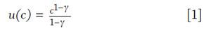
Risk aversion is a concept originally developed by Arrow (1965, 1971) and Pratt (1964), where the goal is to determine some level of constant consumption a person would accept in exchange for a higher average level of consumption with greater variability. Several utility functions are used to estimate risk aversion, but the most common is a constant relative risk aversion (CRRA) utility function, as noted by equation 1, which is the base utility function used for the analysis.
Implied within the CRRA utility function is the law of diminishing marginal utility, whereby negative outcomes (especially extreme negative outcomes) are weighted more heavily than positive outcomes. This model lends itself to retirement income modeling because it heavily penalizes scenarios where the retiree is left destitute when the portfolio is extinguished at old age. The income received by the retiree is both discounted and mortality weighted using this model. This is then compared to the target income goal or liability.
Unlike some models that rely on selecting a specific age of death or a certain retirement period, the probability of surviving to each age is used in this model. The probabilities of surviving to each future age are based on an approach known as the Gompertz law of mortality, which is explained in Appendix 3. The Gompertz approach is used to make changes to mortality expectations for different retiree cohorts, with the expectation of a retiree living longer, on average.
Two statistics were estimated for each scenario to determine the relative efficiency of a given strategy—shortfall risk and residual wealth (see Appendix 2). Shortfall risk is effectively a measure of the “pain” associated with not achieving a target income goal. A retiree who is able to always achieve his or her (or their) retirement income goal across all simulations would have a shortfall risk value of 0 percent (no risk). Higher shortfall risk values would be associated with increasing levels of shortfall, and vice versa.
Residual wealth is the second metric estimated using the preference model. Residual wealth can be thought of as the amount of assets remaining at death that could be passed to the retiree’s heirs, relative to the cost of retirement. Similar to shortfall risk, residual wealth is both discounted and mortality weighted, but unlike shortfall risk, there is no utility function applied; however, in this study, a preference factor was used to determine the relative importance of residual wealth to the retiree.
The key objective of this preference model is to weigh the potential benefits of a given annuity type by way of a decreased likelihood of being destitute later in retirement, compared to the potential loss of wealth for the retiree from the purchase of that annuity. The objective of this paper is not to determine whether or not a retiree should annuitize some portion of wealth, but rather, to provide insight as to whether a DIA or SPIA is the better choice.
Retiree Preferences and Research Assumptions
When determining the optimal annuity type or the optimal allocation to annuities, it is common to vary only a few assumptions, such as a retiree’s preference against a retirement income shortfall, or a retiree’s desire to maximize residual wealth at death. The problem with varying only two preferences is that such an approach ignores the potential impact of varying other assumptions, such as average expected returns, which could materially affect the results of the analysis.
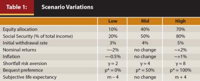
For this analysis, eight different set of assumptions, or retiree preferences, were varied across simulations: (1) initial withdrawal rate; (2) equity allocation; (3) percentage of need covered by Social Security; (4) nominal returns; (5) inflation; (6) life expectancy; (7) shortfall risk aversion; and (8) bequest preference. For each preference or assumption there were three possible values: low, mid, or high. This created 6,561 possible scenarios. Information about the different sets of assumptions or preferences for the scenarios is included in Table 1.
Three equity allocations were considered for the analysis: 10 percent, 40 percent, and 70 percent. The equity portion was effectively modeled as 100 percent U.S. large-cap equities. The non-equity piece (fixed income) was assumed to be 75 percent bond and 25 percent cash. The portfolio was assumed to be rebalanced annually.
An investment management fee of 40 basis points (bps) was included to reflect the general costs associated with investing. Total fees of 40 bps imply a relatively low-cost investing strategy that would predominately feature index funds or low-cost, actively managed funds. The lower the investment fees, the higher the potential benefit of the DIA, because more of the assets are invested in the portfolio in the DIA strategy when compared to the SPIA strategies. The investment management fee was assumed to reduce the annual return for the non-annuitized portfolio in each year of the simulation. Taxes and required minimum distributions for the non-annuitized portfolio were ignored for the analysis.
The impact of an income shortfall on consumption for a retiree household will vary depending on the other sources of guaranteed income the household expects to receive in retirement. For example, a failed portfolio that is providing only 10 percent of a retiree’s income would have a significantly smaller impact on consumption than a portfolio that is providing 75 percent of a retiree’s income. Therefore, Social Security retirement benefits were assumed to be three different percentages of the total income received by the retiree: 20 percent, 50 percent, or 80 percent. Based on data from the Social Security Administration website (www.ssa.gov/pressoffice/basicfact.htm), approximately 50 percent of an average retiree’s income comes from Social Security retirement benefits.
The initial withdrawal rate was the amount withdrawn from the portfolio during the first year of retirement, where that amount was assumed to be increased by inflation each year thereafter for the entire run. This value was assumed to be the target retirement income need for all preference calculations.
The adjustments made to the nominal returns and inflation are noted in Appendix 1. The shortfall risk aversion coefficients apply to shortfall risk calculations in Appendix 2. The bequest preference values apply to the residual wealth adjustments in equation 2.5 (also in Appendix 2). The subjective life expectancy was a reduction in the modal mortality estimate (by four years), using the Gompertz law of mortality.
Considering these different combinations leads to results that are more robust and less dependent on a single set of assumptions or scenario. For example, a higher average inflation assumption is likely to make inflation-adjusted annuities more attractive, and vice versa.
The SPIA purchase amount was assumed to be 50 percent of the portfolio wealth of the retiree couple. The DIA purchase amount was assumed to be 10 percent of the portfolio wealth of the retiree couple. The DIA purchase amount is less than the SPIA purchase, because it creates more income when the benefit finally kicks in. The purchase amount of 10 percent was selected to make the income of the two annuities approximately similar at age 85 for the basic annuity alternatives. The DIA allocation in this analysis was similar to the decumulation benchmark proposed by Sexauer, Peskin, and Cassidy (2012). These authors assumed a 12 percent allocation to a deferred nominal annuity.
Each scenario was based on a 1,000-run Monte Carlo simulation. The stochastic variables were held constant for each specific scenario when testing the eight different annuity types. Therefore, any variation in the resulting benefit from different annuity types was based entirely on the attributes of that annuity type, rather than from the randomness of the simulation.
Probabilities of Success for a Non-Annuity Portfolio
Before reviewing the optimal annuity type for different scenarios, it is worth providing some perspective on the relative safety for a non-annuitized portfolio for the three initial withdrawal rates (3, percent 4, percent and 5 percent), the three equity allocations (10 percent, 40 percent, and 70 percent), the three nominal return assumptions (low, mid, and high), and the three inflation assumptions (low, mid, and high) considered for the analysis. Although the annuity preference model is based on utility, probability of success is a more straightforward way of conveying the relative safety of an initial withdrawal strategy. This approach lends itself more easily to comparisons of past research. The probability of the non-annuity portfolio maintaining a given target income level over a 30-year period, based on the initial withdrawal rate, is included in Table 2 for the 81 different scenario combinations.

The relative safety of an initial withdrawal rate clearly depends on portfolio returns and inflation. Not surprisingly, higher returns and lower levels of inflation tend to result in a higher probability of achieving a retirement goal. The probabilities in Table 2 are generally lower than those noted in past research, especially for the moderate (mid) scenarios. For example, a 4 percent initial withdrawal rate has a 67.4 percent probability of success over a 30-year period based on moderate return and inflation expectations for a 40 percent equity portfolio.
Past research on the “4 percent rule” has generally noted probabilities of success closer to 90 percent over a 30-year period. The lower success rates from this model are largely due to the lower return forecasts, especially the lower initial returns that better reflect bond yields available today. The probabilities of success in Table 2 are slightly higher than those previously noted in research by Blanchett et al. (2013, 2014) primarily due to lower fee assumptions and slightly higher future return expectations used in this study.
Rank Results
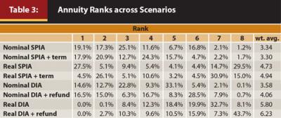
Next, the relative attractiveness of the eight different annuity types will be explored from a ranking perspective. This is the simplest method of contrasting the relative attractiveness of each annuity type. For the rank comparison, the total benefit received (based on the utility preference approach outlined in Appendix 2) for each annuity type is ranked from 1 to 8 for each scenario, where the annuity with the highest benefit receives a rank of 1, and the annuity with the lowest benefit is 8. The percentage of the times each annuity receives each ranking across the 6,561 total scenarios is included in Table 3. Table 3 also includes information on the weighted average rank (wt. avg.), which is just the probability weighted ranking.
Table 3 offers a number of interesting takeaways. First, the nominal SPIA with a 20-year period certain guarantee had the lowest (best) rank, closely followed by the nominal life-only SPIA, and then the nominal life-only DIA. Although the real SPIA had the most 1 rankings (27.5 percent), it also had the second-most 8 rankings (29.5 percent). This suggests the real SPIA works very well in some scenarios, but will likely fare much worse in others. The real DIA options were clearly the worst annuity types among the eight tested, with neither having a single 1 ranking.
Group Results by Preferences and Assumptions
The rank results in Table 3 represent aggregated results across all 6,561 scenarios. Given the obvious dispersion in rankings (for example, the real SPIA), some annuity types clearly work better for a certain set of preferences and assumptions. It would be difficult to demonstrate the relative differences for each of the different scenario combinations individually, given the number of scenarios, therefore, in this section the results are aggregated across each different set of eight assumptions or preferences.
For the aggregation approach, the rankings by annuity type were averaged across all the scenarios that share the same attribute for a given assumption or preference. For example, for the nominal return assumption, one group included all those scenarios with a low return assumption; the second group included those scenarios with a moderate return assumption; and the third group included those scenarios with a high return assumption. The average rank was determined across the 2,217 scenarios for each of the different assumptions or preferences. The results are shown in Table 4.

The relative rank ordering of the annuity types in Table 4 is similar to Table 3, where the nominal SPIA with a 20-year term certain guarantee had the highest average rank, followed by the nominal life-only SPIA, and then the nominal life-only DIA. Certain assumptions, though, clearly had varying degrees of impact on the relative attractiveness of each annuity type. For example, different equity allocations did not significantly change the magnitude of the differences or the relative rank of the eight different annuity types. In contrast, the inflation assumption and the bequest preference significantly impacted the results. For example, a relatively low inflation assumption makes real SPIAs the least attractive annuity type, but a high inflation assumption makes them the most attractive.
The importance of considering different sets of assumptions and scenarios is also apparent based on the ranks in Table 4. For example, an analysis that has a relatively low inflation assumption would find little potential benefits for real SPIAs, while the reverse is true for higher inflation assumptions. Along these same lines, a relatively low bequest preference favors SPIAs, while a relatively high bequest preference favors DIAs.
Relative Benefit Comparison
One problem with the previous grouping approach is that it focuses only a single set of assumptions for each attribute and treats the remaining seven attributes as random (or fixed). This is a problem, because nearly all of the assumptions or preferences will be “known” to the retiree when deciding which annuity type to purchase. For example, a retiree will know what percentage of income he or she will receive from Social Security, how aggressive the portfolio will likely be invested, and what his or her risk aversion is for shortfall risk and residual wealth. Therefore, treating each variable as random does not necessarily allow someone to “zoom in” on the specific annuity that is best given his unique circumstances.
In this section, a slightly different approach is taken to contrast the relative attractiveness of each annuity type, where the relative benefits are compared, based on the benefit calculation approach introduced in Appendix 2. The relative benefit was determined by calculating the difference in the total benefit for the annuity type with the lowest benefit for a given scenario versus each other annuity type. For example, if the minimum benefit across the eight annuity types was 110 percent, and one annuity had a benefit of 120 percent, its relative benefit would be 8.3 percent (formula: ((110%/120%) – 1) = 8.3%).
The average benefit cost is likely a better way to gauge the attractiveness of the annuity types because the differences in benefits were incredibly small for a number of the scenarios (sometime less than .01 percent). Therefore, a rank comparison may not accurately describe the true differences in relative efficiency. This is the case because an annuity may be slightly less efficient for one scenario, yet materially more efficient in another. The annuity may still achieve the same average rank despite the fact the average benefit may be materially highest across both scenarios.
To determine the relative importance of each of the eight assumptions and preferences, a multivariate regression was performed. A multivariate regression is an ideal way to view the relative impact of how one independent variable (the preference or assumption) influences the dependent variable (the benefit), holding all other variables constant.
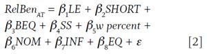
For the relative benefit regression, the relative benefit (RelBen) for a given annuity type (AT) was the dependent variable and was regressed against the eight independent variables included in the analysis: life expectancy (LE), shortfall risk preference (SHORT), bequest risk preference (BEQ), Social Security income weight (SS), initial withdrawal rate (w percent), nominal returns (NOM), inflation (INF), and equity allocation (EQ) based on equation 2. For the regression, each independent variable was assigned a value of 1, 2, or 3 for low, mid, or high values, respectively.
The regression was run for each of the eight different annuity types. The resulting β coefficients provide insight as to the impact of a low, mid, or high value on the relative attractiveness of each annuity type. The results of the regression are included in Table 5.
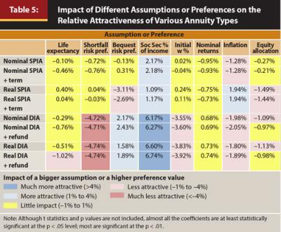
When trying to interpret the β coefficients in Table 5, one perspective is to think of the coefficients in terms of how a bigger assumption or higher preference value changes the relative benefit received from purchasing that annuity type. For example, a bigger assumption for the initial withdrawal rate would result in a higher initial withdrawal rate (for example, 5 percent versus 3 percent). In Table 5, the coefficients for the SPIAs were approximately zero, while the coefficients for the DIAs were approximately –3.7 percent. This suggests DIAs become increasingly less attractive for higher initial withdrawal rates, while SPIAs are not that impacted by initial withdrawal rates.
Table 5 provides an insight as to both the direction and magnitude of different values. For example, the highest absolute values in Table 5 are for Social Security as a percentage of income assumption, where the DIA values average approximately 6.5 percent. This means retirees with a higher percentage of their income coming from guaranteed income sources would find DIAs very attractive. In contrast, underfunded participants are likely to find DIAs materially less attractive.
Another example where the relative attractiveness of DIAs changes is based on different shortfall risk preferences or how a retiree would “feel” about running out of money. The negative values in Table 5 for shortfall risk preference for DIAs are approximately –4.7 percent. Therefore, a retiree who is very concerned about having no money at an older age would find DIAs less attractive than a retiree with a weak or moderate preference.
A More Competitive DIA Marketplace
As the DIA marketplace continues to grow, the products are likely to become increasingly competitive. Seventeen companies provided quotes on nominal SPIAs, and six companies provided quotes for nominal DIAs. This lack of competition likely has a negative impact on the payout rates for DIAs. For example, although New York Life offered the most attractive payout rate for a nominal DIA, its payout rate for the nominal SPIA was approximately 7 percent lower than the highest payout rate available from ING USA Annuity and Life Insurance Co. Therefore, it’s worth considering what may happen if DIA rates become relatively more attractive to SPIAs in the future.
In this section, the entire analysis was redone; however, the payouts for the DIAs were assumed to increase by 5 percent across the board, while the SPIA rates were held constant. For example, the payout for nominal DIAs in the analysis was 34.81 percent; however, for this new analysis the payout was 36.55 percent. Similar to Table 3, the rank results across each of the 6,561 scenarios are included in Table 6 based on the higher assumed DIA payout rates.
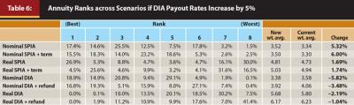
Findings suggest that a slight increase in DIA payout rates causes nominal DIAs to become the most attractive annuity type, on average. However, nominal SPIAs are still a close second. Therefore, while DIAs may currently be suboptimal, on average, across the range of assumptions and preferences considered in this analysis, the difference between DIAs and SPIAs is marginal at best. As competition increases in the DIA space, and relative payouts improve, DIAs are likely to become increasingly competitive.
Conclusions
Results from this study suggest that the relative attractiveness of different annuity types considered varies significantly by scenario and assumptions. Although DIAs work well in certain situations, SPIAs—especially SPIAs with 20-year period certain payments—are the most efficient, on average, across all the scenarios considered. Real SPIAs were the most volatile annuity type from an efficiency perspective, where these products tended to be either the absolute best or absolute worst annuity type. Real DIAs were also the least efficient of the eight annuity types considered. Real DIAs were not optimal in any of the 6,561 scenarios considered, suggesting retirees interested in a DIA may wish to focus on nominal payout versions.
Despite that DIAs are a relatively new, they appear to hold great promise, especially if payout rates marginally improve. For example, if DIA rates were 5 percent higher, they would have been the most attractive annuity type, on average, in this study. DIAs may also represent a more palatable hedge against longevity risk for retirees than traditional annuities, because they are considerably cheaper and therefore provide significantly more liquidity to retirees. In summary, the future is likely bright for DIAs. These annuity products are worth considering when developing an income strategy for retirees.
References
Arrow, Kenneth J. 1965. Aspects of the Theory of Risk Bearing. Yrjö Jahnsson Lectures. Helsinki, Finland: Yrjö Jahnsson Foundation.
Arrow, Kenneth Joseph. 1971. Essays in the Theory of Risk-Bearing, Vol. 2. Amsterdam: North-Holland Publishing Co.
Blanchett, David M., Michael Finke, and Wade D. Pfau. 2013. “Low Bond Yields and Safe Portfolio Withdrawal Rates.” The Journal of Wealth Management 16 (2): 55–62.
Blanchett, David M., Michael Finke, and Wade D. Pfau. 2014. “Asset Valuations and Safe Withdrawal Rates.” The Retirement Management Journal. Forthcoming.
Finke, Michael, Wade D. Pfau, and David M. Blanchett. 2013. “The 4 Percent Rule Is Not Safe in a Low-Yield World.” Journal of Financial Planning 26 (6): 46–55.
Gong, Guan, and Anthony Webb. 2010. “Evaluating the Advanced Life Deferred Annuity—An Annuity People Might Actually Buy.” Insurance: Mathematics and Economics (46): 210–221.
Milevsky, Moshe A. 2005. “Real Longevity Insurance with a Deductible: Introduction to Advanced-Life Delayed Annuities (ALDA).” North American Actuarial Journal 9 (4): 109–122.
Pfau, Wade D. 2013. “Why Retirees Should Choose DIAs over SPIAs.” Advisor Perspectives September 24.
Pratt, John W. 1964. “Risk Aversion in the Small and in the Large.” Econometrica 32 (1/2): 122–136.
Scott, Jason S. 2008. “The Longevity Annuity: An Annuity for Everyone.” Financial Analysts Journal 64 (1): 40–48.
Scott, Jason S., John G. Watson, Wei-Yin Hu. 2007. “Efficient Annuitization: Optimal Strategies for Hedging Mortality Risk.” Pension Research Council working paper 2007-09.
Sexauer, Stephen C., Michael W. Peskin, and Daniel Cassidy. 2012. “Making Retirement Income Last a Lifetime.” Financial Analysts Journal 68 (1): 74–84.
Citation
Blanchett, David. “Determining the Optimal Fixed Annuity for Retirees: Immediate versus Deferred.” Journal of Financial Planning 27 (8) 36–44.