Journal of Financial Planning: February 2015
David M. Blanchett, CFA, CFP®, is head of retirement research at Morningstar Investment Management in Chicago, Illinois.
Acknowledgement: The author thanks Michael Kitces and Hal Ratner for helpful comments and edits.
Executive Summary
- Debate continues regarding how an investor’s equity allocation should change during retirement. This study tests four different changing equity glide path shapes: increasing, decreasing, V-shaped, and -shaped contrasted against the potential benefit of a constant glide path.
- The decreasing glide path was found to be the optimal glide path shape across a wide range of scenarios based on the analysis; however, results showed no clear, one ideal glide path shape for each retiree scenario.
- The increasing glide path was noted to be the least efficient, and the V and shapes fell in the middle.
- The decreasing glide path resulted in approximately 2.0 percent more utility-adjusted overall potential wealth compared to a constant glide path; the increasing glide path resulted in a 2.7 percent overall potential wealth decrease.
- Retiree risk tolerance was not explicitly considered in this analysis. If it was, the decreasing glide path would likely become even more attractive.
There is a growing debate regarding the optimal equity allocation and how it should adjust during retirement. This is the glide path question. While common rules, such as 100 minus your age, still exist, a growing body of research is exploring this issue. Research findings on the optimal glide path shape for retirees has varied, where declining (Bengen 1996), constant (Blanchett 2007), and rising (Pfau and Kitces 2013) glide path shapes have each been recommended based on different models and perspectives.
In this paper, the potential benefit of various glide path shapes will be explored using four changing glide paths: increasing, decreasing, V-shaped, and Λ-shaped. These are contrastedagainst the relative potential benefit of a constant glide path, or one that does not change during retirement.
In this study, the optimal glide path shape is determined using a preference model based on utility. Eight different sets of assumptions, or preferences, are varied for the analysis: (1) initial withdrawal rate; (2) equity allocation; (3) percentage of total retirement income need covered by Social Security; (4) nominal returns; (5) inflation; (6) life expectancy; (7) shortfall risk aversion; and (8) bequest preference. For each assumption, three possible values are possible: low, moderate, or high, for a total of 6,561 scenarios. This approach can lead to conclusions that are more robust than an analysis based on a more limited set of assumptions. An autoregressive return model is used for the analysis that explicitly incorporates today’s low bond yields, where yields are assumed to randomly drift back toward a higher value, which is more consistent with the long-term average, as the simulation progresses.
Understanding Distribution Glide Paths
Various research has explored how equity allocations should change over an investor’s life cycle. Early research by Merton (1969) suggested that an investor’s equity allocation should not change over time based on two relatively limiting assumptions—constant relative risk aversion, and that returns are independently and identically distributed.
Taking a more comprehensive view of wealth has led to recommendations that the equity allocation should vary over the life cycle. For example, Bodie, Merton, and Samuelson (1992) found that greater labor supply or human capital flexibility permits particularly the young investor to hold a higher fraction of financial wealth in risky assets.
Retirement provides an interesting period where investors may seek to change their allocations over time. Bengen (1996) noted that declining glide paths reduced sustainable withdrawal rates; however, the impact was modest and likely optimal when balancing other objectives. Blanchett (2007) found that a constant equity allocation is surprisingly efficient when compared to different types of decreasing glide paths. Pfau and Kitces (2013) suggested a rising glide path may be optimal.
For this analysis, five different glide path shapes are considered: four that change over time and one that remains constant. The selection of these shapes is arbitrary, but meant to capture the different potential shapes that may be considered by a retiree. For each of the four glide path shapes that change over time, the analysis further breaks these into “fast” and “slow” change categories, where the relative change of the fast glide path is twice the change of the slow glide path. Therefore, there are two decreasing glide paths (where the equity allocation decreases during retirement), two increasing glide paths (where the equity allocation increases during retirement), two V-shaped glide paths, and two Λ-shaped glide paths. The final glide path shape is constant, where the equity allocation remains static throughout retirement.
Three different average equity allocations are considered for the analysis: 20 percent, 40 percent, and 60 percent, where the changes are assumed to be made against the base equity allocation. For example, the initial equity allocation for the decreasing fast glide path with a 40 percent base allocation would be 60 percent in year one decreasing to 20 percent by year 40.
The average equity allocation is identical across the nine glide path shapes over the first 40 years of the simulation; that is, equal to the base equity allocation of 20 percent, 40 percent, or 60 percent. The equity allocation after year 40 is assumed to be whatever the equity allocation was in year 40. The different changes to the base equity allocations are shown in Figure 1.
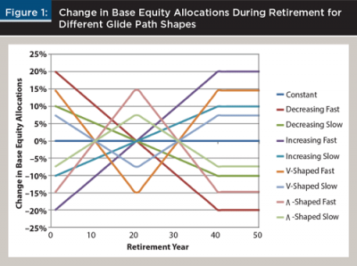
Considerable differences exist in the equity allocations for the different glide path shapes shown in Figure 1. For example, assuming a base equity allocation of 40 percent, the decreasing fast (D_F) glide path would have an equity allocation of 60 percent (40 percent + 20 percent = 60 percent) in year 1, while the increasing fast (I_F) glide path would have an equity allocation of only 20 percent (40 percent – 20 percent = 20 percent) in year 1. More precise increments are not considered beyond slow or fast to ensure a reasonable difference between the different shapes.
Return Simulation Model
The majority of research on sustainable withdrawal strategies has used either historical rolling time periods or a stochastic (Monte Carlo) simulation process for returns, with stochastic simulations being the most common. The returns for stochastic simulations are typically based on long-term historical averages or forecasts, where the expected return of an asset class is the same for each year of the simulation (although the actual return for a given year of a given run would vary stochastically). These approaches are less useful when there is a significant and sustained deviation, such as the current low bond yield market. The implications of low bond yields on retirement portfolios have been explored previously in a variety of papers (Blanchett, Finke, and Pfau 2013, 2014; Finke, Pfau, and Blanchett 2013).
This paper uses an autoregressive return simulation model similar to the one introduced by Blanchett et al. (2013) that incorporates low bond yields, yet assumes yields drift toward a higher value over time. The model used herein is effectively identical to the model used by Blanchett (2014) to analyze the potential benefit of deferred income annuities (DIAs) compared to single premium immediate annuities (SPIAs). This model provides a more realistic method of forecasting returns than assuming the same average return for each year, because recent returns have generally been lower than long-term returns. The order of portfolio returns experienced during retirement is very important. Low initial returns in retirement tend to result in higher probabilities of portfolio sustainability failure. This is an effect commonly referred to as sequence risk.
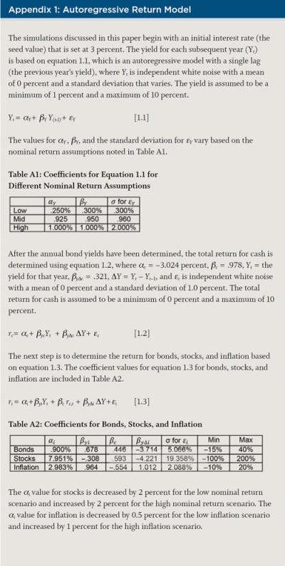
The initial bond yield, which is known as the seed value, is based on current bond yields, and is assumed to be 3 percent. This value is higher than the yield on the Barclays Aggregate Bond Index, which was 2.33 percent as of July 7, 2014, but considerably lower than the long-term average. The initial bond yield sets the “seed” where the future yields change over time, generally trending toward a higher longer-term average as the simulation progresses.
The actual yields experienced within each year of the simulation will also vary over time due to noise in the model. While it is possible that actual bond yields will not revert back toward some higher value, if this does happen there will be material implications not only for this paper, but retirement research in general. The model used to create the expected annual returns for cash, bonds, and stocks, as well as inflation, is explained in greater detail in Appendix 1.
Preference Model
The majority of retirement income research considers retirement consumption from a life cycle perspective, where the implied goal of a retiree is to smooth consumption over his or her (or their) lifetime. Optimal strategies are determined primarily through an approach that incorporates risk aversion (utility), or the likelihood of achieving some goal (the probability of success/failure). Both these approaches have their merits, however an approach that considers risk aversion with respect to the amount of income received is likely a better estimate of individual preferences because it allows for a more “colorful” set of outcomes when compared to the relatively binary nature of whether or not a goal is achieved.
Risk aversion is a concept developed by Arrow (1965, 1971) and Pratt (1964), where the goal is to determine some level of constant consumption a person would accept in exchange for a higher average level of consumption with greater variability. While there are several utility functions used to estimate risk aversion, the most common is a constant relative risk aversion (CRRA) utility function, as noted by equation [1], which is the base utility function used for the analysis.
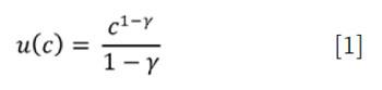
Implied within the CRRA utility function is the law of diminishing marginal utility, whereby negative outcomes (especially extreme negative outcomes) are weighted more heavily than positive outcomes. This model lends itself to retirement income modeling because it heavily penalizes scenarios where the retiree is left with a consumption shock, such as when a portfolio is depleted prematurely. The income received by the retiree is both discounted and mortality weighted using this model. This is then compared to the target income goal or liability.
Unlike some models that rely on selecting a specific age of death, such as age 95, or a certain retirement period, such as 30 years, the probability of surviving to each age is used for the model. These probabilities are based on the Gompertz Law of Mortality, which is explained in Appendix 3.
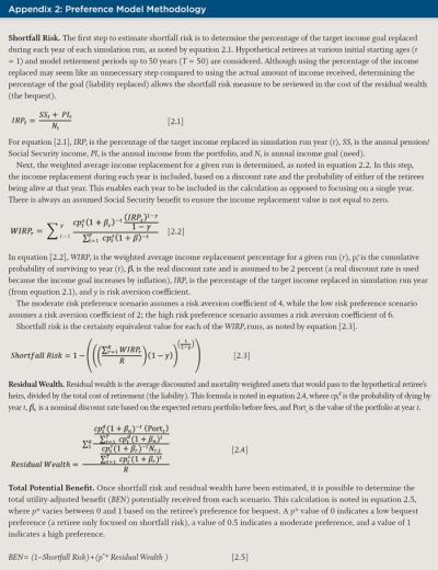
Two statistics are estimated for each scenario to determine the relative efficiency of a given strategy: shortfall risk and residual wealth. The derivation of the metrics is explained in greater detail in Appendix 2.
Shortfall risk is effectively a measure of the “pain” associated with not achieving a target income goal. A retiree who is able to always achieve his or her (or their) retirement income goal across all simulations would have a shortfall risk value of 0 percent (no risk). Higher shortfall risk values would be associated with increasing levels of probable shortfall.
Residual wealth can be thought of as the amount of assets remaining at death that could be passed to the retiree’s heirs, relative to the cost of retirement. Similar to shortfall risk, residual wealth is both discounted and mortality weighted, but unlike shortfall risk there is no utility function applied; however, a preference factor is used to determine the relative importance of residual wealth to the retiree. These values are then combined to get a utility-adjusted wealth (or benefit) measure that can be used to compare strategies.
Retiree Preferences
When determining the optimal retirement income strategy, it is common to vary only a few assumptions, such as the retirement period or the initial equity allocation. The problem with varying only one or two assumptions is that other factors, such as assumptions of average expected returns or a preference against high shortfall risk, can materially affect the results of the analysis.
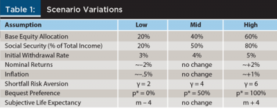
For this analysis, eight different set of assumptions or retiree preferences vary across simulations: (1) initial withdrawal rate; (2) base equity allocation; (3) percentage of need covered by Social Security; (4) nominal returns; (5) inflation; (6) life expectancy; (7) shortfall risk aversion; and (8) bequest preference or the relative importance of residual wealth. For each preference or assumption there are three possible states: low, mid, or high, which creates 6,561 different possible scenarios. Information about the different sets of assumptions or preferences for the scenarios is included in Table 1.
As noted previously, three different base equity allocations are considered for the analysis: 20 percent, 40 percent, and 60 percent. The equity portion is effectively modeled as 100 percent U.S. large capitalization equities, while the non-equity piece (fixed income portion) is assumed to be 75 percent bonds and 25 percent cash. The portfolio is assumed to be rebalanced annually.
An investment management fee of 40 basis points (bps) is included to reflect the general costs associated with investing. Total 40 bps in fees implies a relatively low-cost investing strategy that would predominately feature index funds or low-cost active funds. The investment management fee is assumed to reduce the annual return for the portfolio in each year of the simulation. Taxes and required minimum distributions for the portfolio are ignored.
The impact of an income shortfall on consumption for a retiree household will vary depending on the other sources of guaranteed income the household expects to receive in retirement. For example, a portfolio that fails to maintain a consistent consumption through the entire retirement period that is expected to provide only 10 percent of the retiree’s income would have a significantly smaller impact on consumption than a portfolio that is expected to provide 75 percent of a retiree’s income. Therefore, Social Security retirement benefits are assumed to be three different percentages of the total income received by the retiree: 20 percent, 50 percent, or 80 percent. The average retiree receives approximately 50 percent of his or her income from Social Security retirement benefits, based on data from the Social Security Administration website (www.ssa.gov/pressoffice/basicfact.htm).
The initial withdrawal rate is the initial amount withdrawn from the portfolio during the first year of retirement, where that amount is assumed to be increased by inflation each year thereafter for the entire run. This value is assumed to be the target retirement income need for all preference calculations.
The adjustments made to the nominal returns and inflation are provided in Appendix 1. The shortfall risk aversion coefficients apply to shortfall risk calculations in Appendix 2. The bequest preference values apply to the residual wealth adjustments in equation [2.5] (also in Appendix 2). The subjective life expectancy is a reduction in the modal mortality estimate (by four years), using the Gompertz Law of Mortality.
Considering these different combinations leads to results that are more robust and less dependent on a single set of assumptions or scenarios. For example, a higher average inflation assumption is likely to make inflation-adjusted annuities more attractive. This approach also allows for the relative impact of each preference or assumption to be determined later in the paper through a multivariate regression.
Each of the 6,561 scenarios is based on a 1,000 run stochastic simulation. The stochastic variables are held constant for each specific scenario when testing the nine different glide path shapes. Therefore, any variation in the resulting potential benefit from different glide paths is based entirely on the attributes of that glide path, rather than from the randomness of the simulation.
Probabilities of Success for Various Withdrawal Rates
Although the primary method of determining the optimal glide path is based on a utility model, it is worth first comparing the probabilities of success for the different approaches. Probability of success is a common metric in the financial planning field, especially in past literature when estimating sustainable withdrawal rates. Of course, some of the preference variables or assumptions, such as shortfall risk aversion and bequest preference, have no effect on the probability of success; however, each of the other variables can impact success probability to varying levels.
For simplicity, and to be consistent with the analysis in the remainder of this paper, the probabilities of success for each of the eight changing glide path shapes are contrasted against the probability of success for the constant glide path for various initial withdrawal rates. This is done because what planners tend to be most concerned with is not whether a glide path shape is successful, but rather how successful it is versus its opportunity set.
Table 2 includes the probability of success for the 3 percent, 4 percent, and 5 percent initial withdrawal rates over a 30 year retirement period for the three different base equity allocations for each of the eight changing glide path shape strategies versus the constant glide path shape. The probability of success is estimated by counting the number of runs the portfolio is able to achieve its income and dividing by the total number of runs in the simulation (1,000).
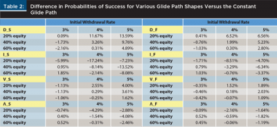
The results shown in Table 2 suggest there are considerable differences in the probabilities of success for varying initial withdrawal rates and different glide path shapes when compared to the constant glide path. For example, for the 40 percent equity portfolio with a 4 percent initial withdrawal rate, the decreasing slow (D_S) glide path had a probability of success that is 3.26 percent higher than the constant glide path. Alternatively, the increasing slow (I_S) glide path had a probability of success that was 8.14 percent lower. This suggests the probability of success of the decreasing slow glide path is 11.40 percent higher than the increasing slow glide path.
It is worth noting the probabilities of success for the decreasing glide path shapes are almost always positive when compared to the constant glide path, while the increasing glide path shapes are more negative. The V-shaped and Λ-shaped glide paths have differences in the probabilities of success that are less than the increasing or decreasing glide paths; however, the V-shaped glide path was slightly better than the constant glide path, while the Λ-shaped glide path was slightly worse. Overall, these findings suggest that glide paths that decrease initially during retirement are potentially better than constant glide paths, and ones that increase initially are potentially worse.
To put the overall success rates in perspective, the probability of success for the 4 percent initial withdrawal rate over 30 years, for the 40 percent base equity allocation with a constant glide path and moderate nominal returns and inflation expectations, is 71.5 percent (versus 73.5 percent for the decreasing fast glide path, and 68.2 percent for the increasing fast glide path). The reason the probability of success is relatively lower for these simulations than in past studies is due largely to the model used to forecast returns, which is an autoregressive model based on today’s low bond yield environment.
Rank Results
In the previous section, the glide paths were contrasted based on their respective probabilities of success over a 30 year retirement period. In this section, the focus is on the relative rank of each approach across the 6,561 scenarios. The rankings are based on the preference model outlined in Appendix 2, which may be a better gauge of how a retiree would feel about an outcome because it incorporates both shortfall risk and residual wealth preferences and the relative magnitude of failure (versus being a simple, bright-line measure).
For the rank comparison, each glide path is ranked from 1 to 8 for each scenario, where the glide path with the highest potential benefit would receive a rank of 1, and the glide path with the lowest potential benefit would be 8. The percentage of times each glide path receives each ranking across the 6,561 total scenarios is included in Table 3. Table 3 also includes information on the weighted average rank (Wt Avg), which is the probability weighted ranking, as well as the average increase in utility-adjusted benefit (when compared to the constant glide path) across all scenarios.

Table 3 offers a number of interesting takeaways. First, the decreasing fast (D_F) glide path was optimal for the majority of scenarios (75.2 percent), while the increasing fast (I_F) glide path was the least optimal for the majority of scenarios (84.5 percent).
The weighted average ranking of the decreasing glide path shapes was the best, with the fast and slow having ranks of 2.33 and 2.57, respectively. Not surprisingly, given these weighted average ranks, the decreasing glide path shape also had the greatest improvement in utility-adjusted potential wealth when compared to the constant glide path shape. For example, the decreasing glide path had an average utility increase of 2.06 percent between fast and slow [(2.68 percent+1.44 percent)/2=2.06 percent], while the increasing glide paths resulted in a loss in a reduction of utility-adjusted potential wealth of –2.74 percent, on average [(–1.74 percent+–3.74 percent)/2=–2.74 percent].
The V-shaped and Λ-shaped glide paths were in between the increasing and decreasing glide paths, and generally consistent with the initial change in shape where V was superior to Λ. Overall, these findings suggest that a decreasing glide path is generally the most optimal for a retiree, while an increasing shape is the least optimal, which is consistent with the probability of success analysis in the previous section.
Relative Benefit Comparison
Some perspective on the relative importance of each of the eight attributes considered in the analysis is provided in this section. In practice, most of the assumptions or preferences will be known by the retiree when deciding which glide path to select. For example, a retiree can take steps to determine what percentage of income he or she can expect to receive from Social Security, how aggressive the portfolio will likely be invested, and what his or her risk preference is for shortfall risk and residual wealth. Therefore, treating each variable as random and averaging the results across all scenarios does not necessarily allow the reader to zoom in on the specific glide path that may be considered optimal given a specific client’s circumstances or preferences.
Similar to the previous section, the relative potential benefits are contrasted using the utility-adjusted benefit measure outlined in Appendix 2. The average benefit cost is likely a more precise way to gauge the attractiveness of the glide paths, because the differences in potential benefits were incredibly small for a number of the scenarios (for example, 99.99 percent versus 99.98 percent). Therefore, a rank comparison may not accurately describe the true differences in relative efficiency, because a glide path may be slightly less efficient for one scenario, yet materially more efficient in another and still have the same average rank. This may be true despite the fact the average benefit may be materially highest across both scenarios.
A multivariate regression was used to determine the relative importance of each of the eight assumptions and preferences.
For the regression, the relative potential benefit (RelBen) for a given glide path shape (GS) is the dependent variable. This regressed against the eight independent variables included in the analysis: (1) life expectancy (LE); (2) shortfall risk preference (SHORT); (3) bequest risk preference (BEQ); (4) Social Security income weight (SS); (5) initial withdrawal rate (w percent); (6) nominal returns (NOM); (7) inflation (INF); and (8) base equity allocation (EQ), based on equation [2]. For the regression, each independent variable was assigned a value of 1, 2, or 3 for low, mid, or high values, respectively, as follows:
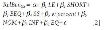
The regression was run for each of the eight different changing glide path shapes. The resulting β coefficients provide insight as to the impact of a low, mid, or high value on the relative attractiveness of each glide path shape. The results from the regression are included in Table 4. Although t statistics and p values are not included in Table 4, any coefficient with an absolute value greater than 0.04 percent is statistically significant at the p < .01 level.
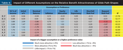
The regression coefficients provide an interesting perspective on the relative importance of each preference or assumption on the relative benefit of a particular glide path. When interpreting the coefficients in Table 4, one perspective is to think of the coefficients in terms of how a larger assumption or higher preference value changes the relative potential benefit received from utilizing that glide path shape. For example, a bigger assumption for the initial withdrawal rate would be a higher initial withdrawal rate, say 5 percent versus 3 percent. Clearly, certain assumptions, such as percentage of Social Security, nominal returns, and bequest risk preference have a much larger impact on the results than other assumptions, such as inflation, life expectancy, and shortfall risk preference.
The increasing fast glide path shape had the highest coefficients on an absolute basis, suggesting it is the glide path shape that will be most sensitive to assumptions used for any type of analysis. The increasing fast glide path will become considerably more attractive for retirees or scenarios in particular where there is a large Social Security benefit, a higher initial withdrawal rate, and a higher initial equity allocation. The increasing fast glide path will become considerably less attractive for retirees or scenarios in particular where there are lower nominal returns or a bequest preference. The bequest risk preference is especially important because an analysis that focuses on metrics like the probability of success, which ignores bequests entirely, is likely to find the increasing fast glide path more optimal, especially on a relative basis. Also, because the increasing fast glide path does relatively poorly in high-return scenarios does not mean it does relatively well in low-return scenarios; in fact, the only scenarios in which it does well are dominated by those with no bequest preference and low withdrawal rates.
Conclusions
This paper provides an overview of the potential benefit of different retirement glide path shapes. The results of the analysis suggest that the actual relative attractiveness of a given glide path is likely to vary by scenario and assumptions; however, decreasing glide path shapes—glide paths where the equity allocation decreases during retirement—appear to be more efficient when compared to the other three changing glide path shapes considered, as well as a constant equity glide path. Findings were relatively robust across the 6,561 scenarios considered, suggesting that even under different assumptions or preferences, the potential benefit of a decreasing glide path is likely to remain.
Although this analysis by no means settles the retirement glide path debate, it does provide some relative perspective. Results suggest that equity allocations should decrease initially during retirement. The relative benefit of a decreasing equity glide path can at least be partially attributed to the return model used for the analysis, which directly takes into account today’s low bond yields but assumes yields eventually drift higher over time. Additionally, while risk tolerance was not included as an explicit assumption in the analysis, it is generally assumed to decrease as an individual ages, which would likely further suggest a benefit from a decreasing glide path.
References
Arrow, Kenneth J. 1965. Aspects of the Theory of Risk Bearing. Helsinki: Yrjö Jahnssonin Saatio.
Arrow, Kenneth J. 1971. “The Theory of Risk Aversion” (pp. 90–120). Essays in the Theory of Risk-Bearing. Chicago: Markham.
Bengen, William P. 1996. “Asset Allocation for a Lifetime.” Journal of Financial Planning 9 (8): 58–67.
Blanchett, David M. 2007. “Dynamic Allocation Strategies for Distribution Portfolios: Determining the Optimal Distribution Glide Path.” Journal of Financial Planning 20 (12): 68–81.
Blanchett, David M. 2014. “Determining the Optimal Income Annuity for Retirees: Immediate versus Deferred.” Journal of Financial Planning 27 (8): 36–44.
Blanchett, David M., Michael Finke, and Wade D. Pfau. 2013. “Low Bond Yields and Safe Portfolio Withdrawal Rates.” The Journal of Wealth Management 16 (2): 55–62.
Blanchett, David M., Michael Finke, and Wade D. Pfau. 2014. “Asset Valuations and Safe Withdrawal Rates.” The Retirement Management Journal. Forthcoming.
Bodie, Zvi, Robert C. Merton, and William F. Samuelson. 1992. “Labor Supply Flexibility and Portfolio Choice in a Life Cycle Model.” Journal of Economic Dynamics and Control 16 (3): 427–449.
Finke, Michael, Wade D. Pfau, and David M. Blanchett. 2013. “The 4 Percent Rule Is Not Safe in a Low-Yield World.” Journal of Financial Planning 26 (6): 46–55.
Merton, Robert C. 1969. “Lifetime Portfolio Selection under Uncertainty: The Continuous Time Case.” Review of Economics and Statistics 51 (3): 247–257.
Milevsky, Moshe A. 2012. The 7 Most Important Equations for Your Retirement: The Fascinating People and Ideas behind Planning Your Retirement Income. Hoboken, NJ: Wiley.
Pfau, Wade, and Michael Kitces. 2013. “Reducing Retirement Risk with a Rising Equity Glide Path.” Journal of Financial Planning 27 (1): 38–45.
Pratt, John W. 1964. “Risk Aversion in the Small and in the Large.” Econometrica: Journal of the Econometric Society 32 (1/2): 122–136.
Citation
Blanchett, David M. 2015. “Revisiting the Optimal Distribution Glide Path.” Journal of Financial Planning 28 (2): 52–61.