Journal of Financial Planning: March 2012
Executive Summary
- Shortfall risk retirement income analyses offer little insight into how much risk is optimal, and how risk tolerance affects retirement income decisions
- This study models retirement income risk in a manner consistent with risk tolerance in portfolio selection in order to estimate optimal asset allocations and withdrawal rates for retirees with different risk attitudes
- We find that the 4 percent retirement withdrawal rate strategy may only be appropriate for risk-averse clients with moderate guaranteed income sources
- The ability to accept greater shortfall probabilities means that risk-tolerant investors will prefer a higher withdrawal rate and a riskier retirement portfolio
- A risk-tolerant client may prefer a withdrawal rate of between 5 percent and 7 percent with a guaranteed income of $20,000
- The optimal retirement portfolio allocation to stock increases by between 10 and 30 percentage points and the optimal withdrawal rate increases by between 1 and 2 percentage points for clients with a guaranteed income of $60,000 instead of $20,000
Michael Finke, Ph.D., CFP®, is an associate professor and Ph.D. coordinator at Texas Tech University (Michael.Finke@ttu.edu).
Wade D. Pfau, Ph.D., CFA, is an associate professor at the National Graduate Institute for Policy Studies in Tokyo, Japan (wpfau@grips.ac.jp).
Duncan Williams, CFP®, is a doctoral candidate at Texas Tech University (Duncan.Williams@ttu.edu).
Studies that estimate shortfall risk in retirement have helped illustrate how portfolio allocation and withdrawal rates affect the likelihood of running out of wealth late in life. This is extremely important to planners and retirees as they decide how best to invest and consume their savings. Shortfall analyses, however, do not provide much insight into how much shortfall risk a client can bear. This study provides a framework that allows a planner to better understand the trade-off between shortfall risk and the risk of not living well in retirement, how risk tolerance affects withdrawal rates, and how a stream of guaranteed income sources from outside the investment portfolio affects both the withdrawal rate and portfolio allocation to equities.
Shortfall risk literature, which began with Bengen (1994), has been the primary lens through which financial planners view retirement income strategies. Advances to this literature include more sophisticated asset return simulation techniques (Spitzer, Strieter, and Singh 2007; Athavale and Goebel 2011), a broader range of return data (Pfau 2010), variable withdrawal strategies related to portfolio performance (Guyton 2004; Bengen 2006), the inclusion of the pre-retirement period (Pfau 2011a), and the impact of market valuations on decumulation strategies (Kitces 2008; Pfau 2011b). A synopsis of the literature is that an optimist might consider withdrawing 5 percent of capital each year, and a pessimist as low as 2 percent or 3 percent depending on return assumptions and expected longevity.
What is missing from the shortfall literature is the consideration of what is lost when withdrawal rates are overly conservative. By emphasizing a portfolio’s ability to withstand a 30- or 40-year retirement, we ignore the fact that at age 65 the probability of either spouse being alive by age 95 is only 18 percent. If we strive for a 90 percent confidence level that the portfolio will provide a constant real income stream for at least 30 years, this means that we are planning for an eventuality that is only likely to occur 1.8 percent of the time. And even that figure assumes that clients are unable to make adjustments to their spending later in retirement. So by relying on standard historical or Monte Carlo simulations to determine a safe withdrawal rate, clients may be unduly sacrificing much of their desired lifestyle early in retirement.
The failure to include a client’s willingness to adjust is an important shortfall of the shortfall literature. A common thread in the analysis is that all failures are counted the same, without regard to when the failure occurred or what percentage of the client’s stated aggregate spending goal was funded. Such an all-or-nothing approach to retirement simulation is inconsistent with the way trade-offs are framed in retirement. In practice, advisers often help their clients prioritize spending goals with basic living expenses, insurance premiums, and debt payments receiving top priority. Other goals, such as travel and vehicle purchases, are scalable and may even be reasonably expected to disappear entirely late in life. Different spending goals have different priorities and importance (Curtis 2006). Some clients may reasonably prefer a higher travel budget in their 60s and 70s, even if it means a higher probability of having to cut back on their dining and vehicle budgets in their 80s. This would be considered failure in most shortfall risk analyses.
If a couple does not have a very strong desire to leave a liquid bequest (or has planned for the bequest through life insurance), the result of relying on standard simulations is that the vast majority will die with a lot of unspent money that they had intended to use to support their lifestyle. Ideally, we would like to include these unspent funds, and the happiness they could have provided if spent, in a calculation that also considers the serious implications of experiencing a shortfall. Fortunately, both can be modeled by using utility theory—the same concept that underlies modern portfolio theory.
Utility theory assumes that we get less satisfaction from each additional dollar spent. The level of risk aversion determines how much less utility we get for each dollar. For example, a risk-averse client will see his or her utility increase less for a given percentage increase in consumption than someone who is risk tolerant. The implication is that risk-averse clients won’t be much happier with retirement income of $80,000 than $60,000, but will be much worse off with income of $40,000 because they value the spending between $40,000 and $60,000 much more than the spending between $60,000 and $80,000. This makes sense in reality because lower levels of spending cover items we may consider necessities, and higher levels of spending may cover less-essential spending. But the extra spending does still provide some enjoyment.
This point is made clearly in a new article by Milevsky and Huang (2011), who estimate optimal retirement withdrawal rates for retirees with varying degrees of risk tolerance. They find that the traditional 4 percent rule is unrealistic for any client who can accept some risk of having to reduce consumption late in life. They term the retiree a “Vulcan” to highlight the theoretical nature of their estimates and suggest that in reality it is often difficult for both the retiree and the adviser to accept any possibility of running out of money. We agree with the philosophy that accepting a greater shortfall risk is difficult in practice, but nonetheless see the value of presenting estimates of how a client should behave based on risk theory in order to provide insight into the sacrifice involved in applying an overly conservative withdrawal rate.
We add to Milevsky and Huang’s study by incorporating a Monte Carlo asset return simulation method introduced in Williams and Finke (2011) to estimate how different portfolio allocations interact with withdrawal rates to produce optimal portfolio/withdrawal rate combinations for varying levels of risk tolerance. In addition, our approach to optimization is more holistic because we consider all of the client’s sources of retirement income, not just the financial portfolio. We describe how a guaranteed income stream, such as Social Security, annuities, or pension income, changes the optimal asset allocation and withdrawal rate choice. This allows an adviser to recommend a more volatile portfolio for clients who have more guaranteed income sources.
Data and Methodology
This study uses bootstrapped simulations from annual data on total returns for U.S. financial markets since 1926 from Ibbotson Associates’ Stocks, Bonds, Bills, and Inflation. The bootstrapping approach, which draws randomly with replacement from the historical annual returns, preserves the historical means, standard deviations, and correlations, but does not otherwise make an assumption about the underlying distribution of returns. Following Bengen (1994), this study uses the S&P 500 Index (large-capitalization stocks) to represent the stock market and intermediate-term U.S. government bonds to represent the bond market. Inflation data are used to calculate real asset returns, real remaining wealth, and inflation-adjusted withdrawal amounts.
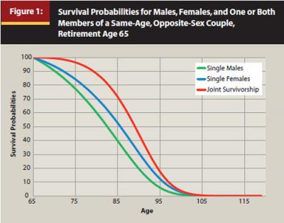
Like Blanchett and Blanchett (2008), but unlike most safe withdrawal rate research assuming a fixed retirement duration, the Milevsky and Huang analysis treats life spans as random, based on actuarial survival probabilities. Our analysis is also based on survival probabilities. We illustrate the framework for a same-age, opposite-sex couple with independent life spans who both retire at age 65. Using data from the Social Security Administration period life table for 2007, Figure 1 shows the probability of survival to each subsequent age, conditional on surviving to age 65, for a single male, a single female, and for at least one member of the couple. From age 65, men have a life expectancy of 17 years to age 82, while women live on average for another 20 years. The longest living member of a couple can expect to live another 24 years to age 89. Considering a traditional 30-year retirement duration assumption, for 65-year-olds the probability of surviving another 30 years to age 95 is 6 percent for males, 12.4 percent for females, and 17.7 percent for at least one member of a couple.
For each of 10,000 55-year simulations of asset returns for stocks and bonds, we calculate the path of remaining wealth from age 65 to the maximum possible age of 119. Upon retiring, accumulated portfolio wealth is assumed to be $1 million. At the beginning of the first year of retirement, an initial withdrawal is made equal to the specified withdrawal rate multiplied by accumulated wealth. Remaining assets then grow or shrink according to the asset returns for the year. At the end of the year, the remaining portfolio wealth is rebalanced to the targeted asset allocation. In subsequent years, the withdrawal amount adjusts by the previous year’s inflation rate, and the order of portfolio transactions is repeated (make withdrawal, experience asset returns, rebalance). No attempt is made to consider fees or taxes. The withdrawal amount is in gross terms, and fees or taxes must be deducted from it. In standard simulation models, if the withdrawal pushes the account balance to zero while either member of the couple is alive, the withdrawal rate was too high, and the portfolio failed. For comparison purposes, we calculate these failure rates for a 30-year retirement duration and for the actual lifetimes of retirees.
Our approach, however, is based on a calculation of expected utility provided by different withdrawal rate and asset allocation strategies. Here we will focus on the intuition for this methodology and include a more mathematical exposition in the appendix. Utility provides a systematic way to evaluate how retirees can decide about the complicated trade-off between spending more early in retirement but increasing the odds of having to spend less later in retirement. At the same time, spend too little and retirees miss the opportunity to enjoy their hard-earned savings but receive the security of knowing the odds for ever exhausting their wealth are quite low. As mentioned, utility analysis also incorporates the idea of diminishing marginal returns—that increasing income levels do not increase happiness at a constant rate. Some people, though, are more aggressive than others in terms of their willingness to accept larger losses for the prospects of potentially enjoying larger gains. Utility accounts for this, as it allows risk-averse individuals to spend less with an emphasis on avoiding bad outcomes, while risk-tolerant individuals may decide to spend more and accept a higher probability of having to cut back later. A risk-tolerant client may be less satisfied with an overly conservative consumption path that more strongly ensures a modest income in retirement without the possibility of living better.
We attempt to evaluate retirement outcomes with these ideas in mind. In determining optimal withdrawal rate and asset allocation combinations, we consider that retirement is supported not only by withdrawals from the financial portfolio but also by other income sources. In our framework, retirees are subjected to two possible future states of consumption: a good one in which the portfolio survives and is able to support consumption on top of the other income sources, and a bad one in which the portfolio is exhausted and only the other sources are available to support consumption. Portfolio withdrawals are kept constant in real terms for as long as wealth remains. Though actual retirees would likely cut spending at some point before their wealth is gone, we do not consider variable withdrawal amounts. No matter the strategy, retirees on track to wealth depletion will experience a lower standard of living than otherwise. We assume that other sources of income are essentially guaranteed and inflation-adjusted, such as Social Security, defined-benefit pensions, or real annuities. Certainly not all pensions and annuities are inflation-adjusted, but this assumption helps to illustrate the key ideas more simply and can be easily modified.
With just two possible spending levels, we can simplify the utility analysis to consider certainty-equivalent dollar amounts. These are the lowest fixed real spending amounts with 100 percent certainty that retirees would be willing to accept to avoid the uncertainty associated with spending more while they still have remaining wealth and spending less when their wealth is gone. Certainty equivalence values are calculated with a formula using the spending amounts when wealth does and does not remain, the probabilities for these two outcomes, and a measure of the retiree’s risk aversion. Whichever strategy provides the largest certainty equivalence is the one that maximizes the retiree’s utility, providing the most satisfactory balance between the trade-offs. We analyze the situation for withdrawal rates between 3 percent and 9 percent, and stock allocations between 0 percent and 100 percent in 10 percentage point increments.
Percentage of Retirement with No Remaining Wealth
We must consider the probabilities for the good and bad spending states. Portfolio success or failure rates provide the standard evaluation tools in traditional safe withdrawal rate studies. But just knowing whether failure takes place at some unspecified point within the couple’s lifetime or over some predetermined retirement duration is not the only important consideration. Rather, retirees may be more interested to know the percentage of their retirement years in which they should expect to make do with no wealth remaining (the bad state). These percentages are weighted by whether one or two members remain alive. Retirees may be more willing to accept failure if it means generally living only one or two years on Social Security than if it means spending 10 years in this predicament.
Figure 2 shows the percentage of time in the couple’s joint lives the couple should expect not to have any wealth. To give some idea about such comparisons, we estimate that with a 5 percent withdrawal rate and a 50 percent stock allocation, a couple faces a 14 percent chance of running out of wealth at some point while at least one of them is alive. Figure 2 shows, however, that this couple should expect to spend only about the final 3 percent of their collective lives with no remaining wealth. More often than not, a widowed female will be the one to endure this outcome. Because these calculations account for the magnitude of failure as well, the optimal stock allocations are generally less than seen with the shortfall risk approach.
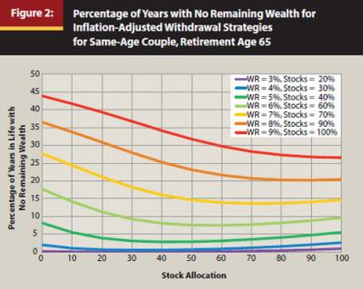
The points identifying the minimal percentages for each withdrawal rate reflect the optimal asset allocation for that withdrawal rate. Though risk-tolerant individuals may be more willing to accept a higher withdrawal rate, and therefore a higher stock allocation, for any given withdrawal rate the optimal asset allocation is fixed across risk-aversion levels. It is the allocation that minimizes the time spent without remaining wealth. Figure 2 also identifies these optimal stock allocations for each withdrawal rate.
Measuring Client Preferences for Income Risk
How will retirees optimize the trade-off between spending more now and increasing the chances of spending less later? A couple’s risk aversion relates to attitudes about withdrawal rates and portfolio failure. In this study, we use a scale that indicates a client’s tolerance for the possibility of a decline in income later in retirement. This relative degree of tolerance or flexibility for retirement income variation is theoretically identical to the tolerance for portfolio volatility prior to retirement. After the client’s tolerance level is assessed, it is a straightforward process to estimate satisfaction from a set of potential retirement outcomes.
We use the concept of certainty equivalence to measure the preference for retirement income paths among clients with a given level of risk tolerance. It is built upon the idea that clients should require a higher expected return for taking on risk. The more risk averse the clients, the higher return they will require to accept a greater possibility of retirement income shortfall. It follows that, given an uncertain income path, a more risk-averse client will be willing to accept a lower certain income than a more risk-tolerant client who prefers a higher income with more possibility of shortfall.
A risk-tolerant retiree will have a coefficient of relative risk aversion closer to 1, and a risk-averse retiree will have a coefficient of relative risk aversion closer to 10. It may be helpful to use shortfall risk probabilities in Figure 2 to estimate a client’s willingness to trade off a higher retirement income (withdrawal rate) for a higher shortfall risk. The risk aversion coefficient is used to assess appropriate withdrawal rate and portfolio allocation combinations for different levels of client risk tolerance.
Figure 3 looks specifically at the case of an aggressive couple with risk aversion of 1 and with a guaranteed income of $20,000. In this figure, certainty equivalence values are shown across the range of asset allocations for withdrawal rates between 3 percent and 9 percent. These risk-tolerant clients can maximize their certainty equivalence with a 7 percent withdrawal rate and a 70 percent stock allocation. This provides their optimal balance between higher income now and less later. Also interesting to note about this figure, an aggressive couple forced to maintain a stock allocation of approximately 35 percent is indifferent between a high income path of $110,000 in two-thirds of retirement years (and a much lower income of $20,000 for about one-third of retirement years) and spending $60,000 for about 99.5 percent of the time and $20,000 in the other 0.5 percent of retirement. That a retiree would maximize his or her utility with a 7 percent withdrawal rate and a 70 percent stock allocation is quite striking in terms of the traditional shortfall risk approach. This strategy would be considered a failure in the traditional shortfall analysis because the portfolio would be exhausted in 57 percent of 30-year retirement durations, and in 43 percent of the actual lifetimes of retiring 65-year-old couples. However, given the clients’ willingness to cut back later in retirement, it produces the optimal solution in terms of projected retirement income paths.
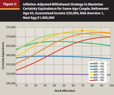
Figure 4 repeats this exercise for a more risk-averse couple with a coefficient of 4. Showing the important role of risk aversion, in this case the couple would choose a withdrawal rate of 4 percent with a stock allocation of 30 percent to maximize utility and certainty equivalence ($57,451). There are fewer cross-over points (which provide the same expected utility) in this case, except that we can see that the couple is indifferent between a 3 percent and 5 percent withdrawal rate for asset allocations of 20 percent and 90 percent stocks.
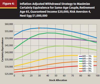
Figure 5 relates the decision between withdrawal rates and risk aversion when the optimal asset allocation for each withdrawal rate is combined with a guaranteed income of $20,000. This figure again details how greater risk tolerance supports higher withdrawal rates. The shortfall risk approach does not tell the whole story by not considering the role of risk aversion.
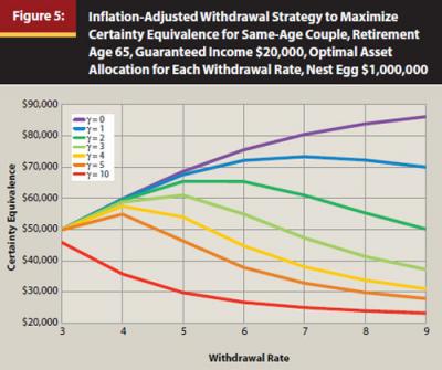
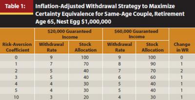
Table 1 repeats the scenario in Figure 5, showing the optimal strategies for income sources of $60,000 as well. This additional income security allows for higher withdrawal rates, generally by about one percentage point, because it is less damaging if wealth is depleted. Even the hyper-conservative retiree with a coefficient value of 10 found a means to prefer a 4 percent withdrawal rate over 3 percent.
Conclusion
This study adds to the retirement decumulation literature by estimating optimal withdrawal rates and asset allocations for retirees with different attitudes toward shortfall risk. We find that a risk-tolerant retiree is willing to accept an increase in shortfall risk in order to spend more in retirement. A greater income stream from Social Security, pensions, or annuities increases both the optimal withdrawal rate and allocation toward risky assets.
We find that the traditional shortfall literature recommendations of a 4 percent withdrawal rate and modest (30 percent) stock allocation are optimal for risk-averse retirees who must revert to living only on Social Security income if they run out of retirement assets. A highly risk-tolerant retiree with only Social Security will optimally choose a higher (7 percent) withdrawal rate and a 70 percent stock allocation. A greater guaranteed income of $60,000 increases the optimal withdrawal rate of both risk-tolerant and risk-averse retirees by about one percentage point.
For planners, the most significant insight is that a client’s willingness to take portfolio risk before retirement is equivalent to a willingness to accept shortfall risk after retirement. A risk-averse investor should choose a lower withdrawal rate in order to reduce the probability of having to reduce consumption later in retirement. This result is similar to the findings of the typical shortfall minimization strategy; however, the traditional approach fails to capture the preferences of a client who is willing to accept the risk of a diminished income in order to live better in retirement. The authors recognize that it may be difficult to consider a strategy that results in an increased shortfall risk; however, it may be helpful to encourage a client to choose among possible conservative strategies (say, between 4 percent and 6 percent) by articulating the shortfall risk/lifestyle return trade-off.
By increasing the size of the income floor in retirement, for example by investing a portion of assets in a guaranteed income product, an adviser is able to recommend both a higher asset decumulation rate and greater portfolio risk. In other words, a client will be better off with a riskier portfolio when the downside drop in spending is not as severe. The magnitude of guaranteed income may then be viewed as a client’s decumulation risk capacity. A larger pension or other source of annuitized income provides a cushion against the loss in quality of life if investment returns are unfavorable or the client outlives his or her assets. Advisers seeking a way to increase expected return in retiree portfolios may be best served by looking into the advantage of mixing a risky investment portfolio with products that protect a minimum level of income.
The economic framework used in this paper provides a scientific approach to a philosophical issue that has long been discussed in the planning community. Practitioners are often torn between a strict interpretation of the safe withdrawal guidance and a looser interpretation that allows retired clients to spend more on things that bring meaning to their lives while accepting greater risk. The implications of the analysis in this paper can give practitioners a framework from which they can engage clients in conversations about sensible trade-offs in retirement.
References
Athavale, Manoj, and Joseph M. Goebel. 2011. “A Safer Safe Withdrawal Rate Using Various Return Distributions.” Journal of Financial Planning 24, 7 (July): 36–43.
Bengen, William P. 1994. “Determining Withdrawal Rates Using Historical Data.” Journal of Financial Planning 7, 4 (October): 171–180.
Bengen, William P. 2006. Conserving Client Portfolios During Retirement. Denver: FPA Press.
Blanchett, David M., and Brian C. Blanchett. 2008. “Joint Life Expectancy and the Retirement Distribution Period.” Journal of Financial Planning 21, 12 (December): 54–60.
Curtis, Robert. 2006. “Monte Carlo Mania.” In Retirement Income Redesigned: Master Plans for Distribution. Harold Evensky and Deena B. Katz, eds. New York: Bloomberg Press.
Guyton, Jonathan T. 2004. “Decision Rules and Portfolio Management for Retirees: Is the ‘Safe’ Initial Withdrawal Rate Too Safe?” Journal of Financial Planning 17, 10 (October): 54–62.
Ibbotson, Roger G., M.A. Milevsky, P. Chen, and K.X. Zhu. 2007. Lifetime Financial Advice: Human Capital, Asset Allocation, and Insurance. Charlottesville, VA: The Research Foundation of the CFA Institute.
Kitces, Michael E. 2008. “Resolving the Paradox—Is the Safe Withdrawal Rate Sometimes Too Safe?” Kitces Report (May).
Milevsky, Moshe A. 2006. The Calculus of Retirement Income: Financial Models for Pension Annuities and Life Insurance. New York: Cambridge University Press.
Milevsky, Moshe A., and Huaxiong Huang. 2011. “Spending Retirement on Planet Vulcan: The Impact of Longevity Risk Aversion on Optimal Withdrawal Rates.” Financial Analysts Journal 67, 2 (March/April): 45–58.
Pfau, Wade D. 2010. “An International Perspective on Safe Withdrawal Rates from Retirement Savings: The Demise of the 4 Percent Rule?" Journal of Financial Planning 23, 12 (December): 52–61.
Pfau, Wade D. 2011a. “Safe Savings Rates: A New Approach to Retirement Planning over the Life Cycle.” Journal of Financial Planning 24, 5 (May): 42–50.
Pfau, Wade D. 2011b. “Can We Predict the Sustainable Withdrawal Rate for New Retirees?” Journal of Financial Planning 24, 8 (August): 40–47.
Poterba, J., J. Rauh, S. Venti, and D. Wise. 2005. “Utility Evaluation of Risk in Retirement Savings Accounts.” In Analyses in the Economics of Aging. D. Wise, ed. Chicago: University of Chicago Press. 13–52.
Spitzer, John, Jeffrey Strieter, and Sandeep Singh. 2007. “Guidelines for Withdrawal Rates and Portfolio Safety During Retirement.” Journal of Financial Planning 20, 10 (October): 52–59.
Williams, Duncan, and Michael Finke. 2011. “Determining Optimal Withdrawal Rates: An Economic Approach.” Retirement Management Journal 1, 2 (Fall): 35–46.
Acknowledgments: We are grateful for comments and suggestions from Dan Moisand, Michael Kitces, Joseph Tomlinson, Francois Gadenne, and Bob Powell. Pfau also thanks financial support from the Japan Society for the Promotion of Science Grants-in-Aid for Young Scientists (B) # 23730272.