Annuitized Income and Optimal Equity Allocation

Journal of Financial Planning: November 2018​

 

 

David M. Blanchett, Ph.D., CFA, CFP^®, is head of retirement research at Morningstar Investment Management. He is a recipient of the Journal’s 2007 Financial Frontiers Award and its 2014 and 2015 Montgomery-Warschauer Award.

 

 

Michael Finke, Ph.D., CFP^®, is chief academic officer at The American College of Financial Services. He is a recipient of the Journal’s 2013 and 2014 Montgomery-Warschauer Award, and the 2017 CFP Board Academic Research Colloquium Best Paper Award in Investments.

Executive Summary

• Prior studies have confirmed that annuitized income such as Social Security or a pension increases the optimal stock allocation of a household’s investment portfolio.

• Buying an income annuity should change the optimal allocation of the remaining investment portfolio. This analysis helps advisers understand how much the remaining equity allocation should change when an annuity is purchased.

• This paper used current annuity and bond prices to estimate the optimal equity allocation for retirees with varying levels of guaranteed income who have higher and lower preference for income stability and bequests. Results indicate that increasing annuitized income has a strong impact on optimal equity allocation in the remaining investment portfolio.

• Results suggest that advisers considering recommending the purchase of an income annuity should primarily draw from bond assets to maintain an appropriate risk level for the investor’s total wealth.​​

Buying an income annuity with a portion of a retiree’s retirement portfolio, or partial annuitization, efficiently reduces the risk of outliving safe investments when funding less flexible spending goals. The non-annuitized portfolio can then be used to achieve an equity risk premium when funding more flexible spending goals. Investment assets can also be used to maintain liquidity for uncertain spending needs or bequests. 

After placing a portion of a retirement portfolio into an income annuity, how should an adviser prudently invest the remaining portfolio? Because a fixed immediate (or deferred) income annuity is constructed by an insurance company using a portfolio of bonds, intuition may suggest that the annuity should be purchased from the bond, or safe asset, portion of a portfolio. However, there is no established best practice for asset allocation when an adviser partially annuitizes a retirement portfolio. 

The goal of this paper is to estimate the optimal asset allocation to stocks and bonds following the purchase of an annuity.

A simple strategy of buying the annuity with bonds would result in an investment portfolio that appears riskier. For example, if an adviser buys a $125,000 income annuity from a $1 million portfolio with a 50/50 allocation to bonds and stocks, the remainder of the portfolio would consist of $375,000 in bonds and $500,000 in stocks (or a 59 percent equity allocation). But is this partial annuitization portfolio reallocation to 59 percent equities as safe as a 50 percent equity allocation within a non-annuitized, investments-only portfolio if the goal is funding retirement income?

This analysis sought to solve for the optimal equity allocation given different levels of annuitization using a utility framework, and to report the resulting equity allocation.

The results of this analysis show that the substitution of an annuity for bonds will reduce the income risk of the remaining portfolio, even though that portfolio has a higher allocation to equities. Higher levels of guaranteed income generally result in riskier optimal client portfolios, consistent with the bond-like nature of guaranteed income; however, the actual portfolio impact varies considerably based on the situation and preferences of the investor.

Partially Annuitized Portfolios

Household portfolios are considered optimal when the allocation of risky assets provides just enough variance in future consumption to be worth the benefit from a higher expected return. Traditional portfolio theory considers a two-asset portfolio of diversified risky assets and risk-free investments (Roy 1952; Tobin 1958; Markowitz 1991). The optimal mix of risky assets depends on a client’s risk aversion. Clients with a higher coefficient of relative risk aversion prefer to hold a higher percentage of their portfolio in risk-free assets, and more risk-tolerant clients prefer to hold a higher allocation of risky assets (Cass and Stiglitz 1970).

More risk results in higher portfolio variance. Higher variance in the payout on investment assets leads to greater volatility in spending. Risk-averse investors prefer greater consumption certainty and are willing to forego a higher expected portfolio return to reduce variation in future spending. In theory, investors and their advisers select the allocation that provides the highest expected utility over time.

This assumes that the client and adviser are investing for spending goals that have a defined time horizon. Retirement complicates the investment portfolio decision because the time horizon is unknown. Consumption volatility can occur because of both investment volatility and variance in longevity, or the risk of outliving assets.

Davidoff, Brown, and Diamond (2005) showed that an investor who wishes to fund income in retirement would maximize their utility by placing a healthy percentage of their savings in an annuity, even if they have some bequest motive. The possibility of running out of money could lead to a big decrease in spending, resulting in a significant reduction in welfare (utility). Milevsky, Moore, and Young (2006) referred to this risk as the probability of financial ruin that occurs when the retiree runs out of money. Because they provide an income floor on top of Social Security, annuities reduce the utility consequence of running out of money through a guaranteed lifetime income that ensures a higher level of minimum spending.

Substituting Income Annuities for Bonds

Many advisers work with clients to establish an acceptable failure rate from a retirement withdrawal strategy. For example, a client and adviser may decide that a 5 percent failure rate is acceptable. All else equal, a retiree who invests a dollar in a fairly priced income annuity, rather than in a bond whose duration is matched to a safe spending need in retirement, will be able to spend more each year at the same failure rate because of the mortality credits provided by the annuity. Insurance company expenses will affect how much of the mortality credits the annuitant will capture.

Pfau (2015) referred to income annuities as “actuarial bonds.” Annuities can be viewed as a bond investment pooled with other retirees (the actuarial part) that provides protection against the risk of outliving assets unavailable with a non-annuitized bond investment. Pfau suggested that an efficient retirement portfolio strategy involves substituting some, if not all, of a retiree’s bond investments for income annuities, depending on the client’s need for liquidity.

When asset returns are known at retirement (e.g., if the retiree creates a bond ladder from existing savings), the likelihood of ruin is affected by the probability that one will live longer than the last bond payment. Bond ladders may provide a useful lens through which to also view the benefit of annuitization, since annuities will provide a higher expected income per dollar spent if the retiree lives longer than the average predicted by insurance company actuaries (assuming expenses on income annuities are modest, which they appear to be (Blanchett 2016)).

A retiree who builds a bond ladder is exposed to greater risk of ruin and a lower expected income if they build the ladder to last beyond expected longevity (Kitces 2015). The longer the length of the bond ladder, say to age 95 or 100, the lower the probability of ruin but the higher the expected income gain from annuitization.

Annuitization allows the retiree to spend as if they have a time horizon equal to slightly longer than the average longevity (how much longer is determined by insurance costs). This means that if the annuity is fairly priced, the cost of the bond ladder to a retiree will be higher because the bond ladder must be constructed to last to an age at which the client assumes an acceptably small failure rate. A safe bond ladder must be constructed to last well beyond the average longevity. If the ladder is built to a 5 percent probability of failure, the annuity will provide a higher income for the same initial investment and will last until death.

Figure 1 shows the potential benefit of annuitization based on the Society of Actuaries individual annuity mortality table¹ to illustrate the distribution of ages at which the surviving spouse is predicted to die, where independence is assumed between spousal mortality rates. The yield curve on nominal Treasury bonds² was used to estimate the cost of creating a bond ladder to provide income for various periods, as of September 1, 2017. 

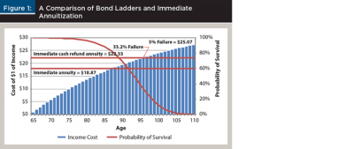
Annuity prices were estimated by taking the average of the top five quotes for a $100,000 joint and survivor immediate income annuity from CANNEX (cannex.com​), an organization that supports the exchange of pricing information for annuity and bank products in North America. The annuity quotes were for a life only annuity and one that includes a cash refund provision. A cash refund provision ensures that the annuitant will at least receive the $100,000 paid for the annuity no matter what age of death (if he or she dies before receiving $100,000 in premium dollar, the insurance company will refund the difference between $100,000 and the income already paid).

An adviser who uses a bond ladder to create income in retirement first needs to specify the age of the last payment, or how many years the bond ladder will last. The curved line in Figure 1 represents the probability that one member of a healthy couple will still be alive at a given age. A ladder built to age 95, for example, will last long enough to provide income for about 57 percent of couples (based on annuity mortality tables) and will be exhausted prior to the death of the surviving spouse for 43 percent of couples. This risk is unacceptable for most clients.

If a retiree were to create a $100,000 bond ladder that lasted long enough to fund spending for 95 percent of couples, building the bond ladder would cost $25.07 per dollar of income (the summed present value of funding an annual $1 income flow between age 65 and 102). If they purchased an income annuity at today’s rates (according to CANNEX data), they would pay $18.87 per dollar of income and have a close to 100 percent chance (assuming a non-zero probability of insurance company default and failure of state guarantee associations as a backup) of funding spending over the couple’s lifetime.

For a retiree concerned about not living long enough to get their money back on the annuity purchase, a joint and survivor annuity costs $22.33 per dollar of income. Had the retiree instead invested $22.33 in a bond ladder, the couple would have a 33.2 percent chance of outliving their savings. Buying an income annuity instead of a bond ladder may allow a retiree to pay less for a safer income.

If the optimal retirement portfolio involves substituting some percentage of bonds with income annuities if the client values lifetime income, what should the rest of the portfolio look like?

Economic analyses have historically considered annuitized income such as Social Security to be an important component of overall wealth (Cocco, Gomes, and Maenhout 2005). Jennings and Reichenstein (2001) showed that the optimal portfolio of a household with a military pension should be more heavily weighted toward stocks than a household that is not eligible to receive a pension. When the value of a bond-like asset such as Social Security or human capital is considered, the optimal stock allocation in the remaining investment portfolio rises. The purchase of a bond-like income annuity suggests that the rest of a retiree’s portfolio should, in fact, be more heavily weighted toward equities to provide the same amount of consumption risk as a non-annuitized portfolio. If a 60 percent bond/40 percent equity portfolio was appropriate for a moderately risk-averse retiree, what would happen if they invested half of their bond portfolio in an income annuity?

Finke and Pfau (2015) considered the annuity to be simply a bond portfolio held within an annuity wrapper and adjusted the remainder of the portfolio accordingly. Following this approach implies that their total financial asset portfolio would now be 30 percent annuities, 30 percent bonds, and 40 percent equities. Their balance sheet, however, would now show a 57 percent equity allocation rather than a 40 percent equity allocation. Their 57 percent equity portfolio would appear riskier when, theoretically, it would pose less retirement income risk than a non-annuitized 40 percent equity portfolio.

The goal of this paper is to move beyond the assumption made by Finke and Pfau (2015) and estimate the actual optimal asset allocation to stocks and bonds following the purchase of an annuity.

Annuities in the Balance Sheet

In order to assess the portfolio consequences of buying an income annuity with investment assets, it is important to understand that retirees already have considerable annuitized wealth. According to 2016 data from the Investment Company Institute,³$10 trillion of the total $25 trillion in U.S. retirement assets is in defined benefit plans and annuities. This figure does not include the value of government pension benefits, such as Social Security retirement benefits, which the authors estimated to be approximately $8 trillion alone for retirees currently in payout status. The value of Social Security benefits for individuals not yet receiving benefits would likely more than double the total estimated value. Therefore, at least half of total assets that are going to be used to fund retirement are already in some form of guaranteed income.

This analysis begins by accounting for the value of annuitized assets most households already have on their balance sheet, for example Social Security. To determine the value of a stream of guaranteed income, the mortality-weighted net present value of future guaranteed income retirement benefits (VI_t) must be estimated. A variety of key assumptions are important when running these estimates, such as the benefit payment amount (GI_t), the age the benefits start (n), the age the benefits end (D), the probability of surviving to the respective age (q_D–n), whether or not there is a cost of living adjustment (COLA_t), and the discount rate (r_t).

The formula used to estimate this is shown as equation 1.

The discount rate for any kind of net present value calculation should reflect the riskiness of the cash flows, where safer cash flows would use a lower discount rate. For example, when estimating the value of Social Security retirement benefits, Treasury bonds would likely be a suitable discount rate. Although counterparty risk exists for annuities, insurers’ reserves and state guarantees suggest a discount rate of corporate bonds at a duration that matches the cash flow duration of the annuity. This assumption is conservative, because regulation of insurance reserves is strict enough that these reserves are likely safer than an average corporate bond portfolio. The longer duration of deferred annuities would require a higher discount rate assuming a positive term premium.

The analysis here used the Treasury yield curve for discount rates and the Society of Actuaries 2012 immediate annuity mortality table⁴ for mortality rates. Ideally, the discount rate should vary by the safety of guarantor of the guaranteed income, and mortality should vary based on the investor; therefore, these calculations are imperfect estimates.

The analysis assumed three household scenarios: single male, single female, or a joint couple (male and female both the same age). For the joint benefit, payments were assumed to continue without decreasing when the first spouse passed away (this is called a 100 percent survivor benefit). This is consistent with how private pensions and annuities with a 100 percent spousal continuation benefit tend to work, but it is different from Social Security retirement benefits, because the surviving spouse typically receives the larger of the two individual benefits.

Using the data in Table 1, an adviser can estimate the approximate portfolio value of a guaranteed income source. For example, a married couple (male and female) both age 65 with a pension benefit that increases annually with inflation and starts immediately would have a multiplier of 25.7. If the expected annual income benefit was $50,000 (combined), the portfolio value of this benefit would be $1.285 million.

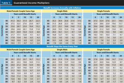
Including the present value of annuitized income as part of a holistic balance sheet allows an adviser to better understand the resources that can be used to meet an income goal in retirement. When a retiree purchases an annuity, this does not mean that their ability to meet their goals has been reduced by the decrease in the value of their investible assets. Assets only have value because they can be used to meet the future spending and legacy needs of clients.

Optimal Equity Allocation and Guaranteed Income

To understand how holding annuitized wealth affects the safety of a retirement plan, an analysis was conducted to determine how the optimal equity allocation for a retiree household should change for a variety of situations and preferences. The base case scenario for the analysis was a couple, male and female, both age 65. The use of a single household type allows one to more easily evaluate the impact of adjusting different model parameters.

Mortality rates were based on the Society of Actuaries (SOA) 2012 Immediate Annuity Mortality Table.⁵ This mortality table was used instead of the Social Security Administration’s 2014 Period Life Table,⁶ because individuals who receive financial planning services tend to be wealthier than the average investor (Martin and Finke 2014). The SOA table is more applicable to individuals and households with higher incomes because they have longer life expectancies, on average. For example, Chetty et al. (2016) noted that the life expectancy of a 65-year-old in the top household income quintile is approximately three years longer than the median life expectancy. This is the same approximate increase in life expectancies when comparing the Society of Actuaries 2012 Immediate Annuity Mortality Table to the Social Security Administration’s 2013 Period Life Table for a 65-year-old.

Instead of modeling a single fixed retirement period (30 years, for example), the retirement model weights the probability of the retiree household surviving to each age. As noted by Blanchett and Blanchett (2008) and others, true success is a portfolio providing income for the life (or lives) of the retiree household and not over some arbitrary fixed period. To provide some perspective on the distribution of mortality in the simulations, there is a 43 percent chance that at least one member of the couple (or both) will survive 30 years in retirement, a 16 percent probability of surviving 35 years, and a 3 percent probability of surviving 40 years.

The guaranteed income benefit for the analysis was assumed to increase annually with inflation for the entire period of the projection. This is slightly different than how actual Social Security retirement benefits work, where the surviving spouse receives the larger of the two benefits upon the death of the first spouse (not both benefits). The approach used for this model would be most consistent with an annuity that includes a cost-of-living adjustment tied to inflation and a 100 percent survivor continuation benefit upon the death of the first spouse.

The retirement income goal was assumed for convenience to be a combination of nondiscretionary and discretionary income goals (50 percent each). For the nondiscretionary portion of the income goal, the annual income need was assumed to increase each year based on inflation. This withdrawal amount was fixed regardless of the ongoing sustainability of the withdrawal amount. In other words, even if the portfolio was headed for certain ruin, that amount would still be withdrawn. For the discretionary portion of the income goal, the annual withdrawal was determined so that the funded ratio for the retiree was constant throughout retirement. The model used to estimate the dynamic withdrawal amount was identical to the approach introduced in Blanchett (2015).

A portfolio fee of 50 basis points was included to reflect modest investment management expenses. While the assumed fee was higher than the costs associated with investing in low-cost index mutual funds (which can be as low as about 5 bps today), it was lower than the fees associated with actively managed mutual funds (which can exceed 100 bps) and/or adviser asset management fees.

Each scenario test was based on a 1,000-run Monte Carlo projection where each run was assumed to last a maximum of 50 years (age 115 for the base case scenario). For each projection, initial withdrawal rates from 1.0 percent to 10.0 percent were considered in 0.1 percent increments (giving 91 test withdrawal rates). Taxes and required minimum distributions were ignored for simplicity. The following sections detail additional key assumptions for the model.

Utility Model

According to economic theory (Modigliani 1966), spending about the same amount each year in retirement provides the greatest satisfaction. A retiree’s willingness to be flexible in terms of annual spending is conceptualized through the slope of the utility function, also known as the coefficient of relative risk aversion (Finke, Pfau, and Williams 2012). Although several utility functions can be used to estimate risk aversion, the most common is a constant relative risk aversion (CRRA) utility function, shown in equation 2, where the amount of utility (U) received varies depending on level of consumption (c) and level of investor risk aversion (y).

Implied within the CRRA utility function is the law of diminishing marginal utility, in which losses (especially extreme losses) are weighted more heavily than gains. This function lends itself to retirement income modeling since it heavily penalizes scenarios where the retiree is left destitute.⁷ A utility model is especially useful for retirement income modeling because it can incorporate a variety of preferences, such as a retiree’s desire to have a more stable lifetime income.

The utility model used for this analysis is similar to the model introduced by Blanchett and Kaplan (2013), where the risk tolerance parameter and the elasticity of intertemporal substitution (EOIS) parameter were treated as separate. This is a recursive utility approach similar to the model introduced by Epstein and Zin (1989). The model is described more fully in the appendix.

Return Assumptions

This analysis used forecasted returns based on Morningstar Investment Management’s 2016 capital market assumptions. Monte Carlo was used to accurately model the impact of cash flows on a portfolio subject to random returns. These forecasted returns are time-varying, where the average returns in early retirement were assumed to be relatively low to reflect current market conditions, but were assumed to drift back toward the long-term average later in retirement.

The historical returns were not assumed to be time-varying (they were constant over the entire projection). For simplicity purposes, the standard deviations and correlation values were the same for both sets of assumptions. There was no assumed serial correlation of returns. The assumptions for the respective series are shown in Table 2. Returns were assumed to be normally distributed for the analysis, and they were generated using the values noted in Table 2.

Equity Allocation Glide Path

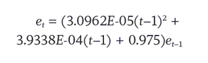
The equity allocation was assumed to decline each year during retirement consistent with the rate of change in the equity allocations for the Morningstar Lifetime Indexes.⁸ Although there has been debate about the efficacy of declining glide paths during retirement, this remains the most common shape among retirement income products today. Equation 3 was used to create the slowly declining equity glide path in which the equity portfolio in percentage (e_t) in each year t of retirement is a function of the allocation in the previous year

​(t –1), with annual rebalancing back to the target allocation.

This approach treats risk aversion associated with the portfolio of assets as separate from the risk aversion associated with income. Although the two may likely be related for some investors, other retirees will be willing to take substantial risk in their portfolio but may be far more risk averse with respect to funding retirement. This model allowed for these varying preferences.

Results

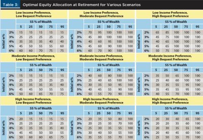
Nine base cases were provided with three income stability preferences and three bequest preferences. Within each case, 25 scenarios varied by initial withdrawal rate and the percentage of a household’s wealth that was held in annuitized income. Retirement wealth was assumed to consist of two assets: annuitized income and the portfolio. Each dollar of annuitized income had a mortality-weighted net present multiple of 25.7, which is the present value of $1 of inflation-adjusted income for life weighted by mortality.

For example, if a retiree household expected $50,000 in annual inflation-adjusted guaranteed income, the value of the annuitized income would be $1,285,000 ($50,000 x 25.7 = $1,285,000). If that household had retirement savings of $500,000, then the total value of the annuitized income would be 71.99 percent of the total wealth for that household ($1,285,000/$1,785,000 = 71.99 percent). Other assets that could potentially be used to fund retirement, most notably home equity, were ignored in this analysis because less than 10 percent of seniors plan to use home equity for retirement living expenses (Munnell, Aubrey, and Soto 2007). Equity allocation represented the percentage of invested, non-annuitized wealth that should optimally be held in equity investments.

Table 3 includes the optimal equity allocations for scenarios that vary by level of annuitized wealth, initial withdrawal rate at retirement, income preference, and bequest preference. The optimal equity allocation at retirement tended to increase at higher levels of guaranteed income, in some cases dramatically. For example, for an investor with a moderate income and bequest preference using a 4 percent withdrawal rate, the optimal equity allocation with 5 percent of wealth in guaranteed income was 30 percent, while the optimal equity allocation with 75 percent of wealth in guaranteed income was 95 percent.

Portfolio Impact of an Annuity Purchase

The previous analysis provided some guidance on how much of the cost of an annuity should be paid from fixed income or equity investments, however it assumed the portfolio and guaranteed income streams had equivalent value to an investor. Because there may be variation among investors in the welfare of annuitized income at market prices, it makes sense to conduct a similar analysis based on the purchase of an actual annuity.

Annuity quotes were obtained from CANNEX on January 6, 2017 for a heterosexual couple both age 65, with a 100 percent continuation benefit, a full cash refund, and no cost-of-living adjustment (the features most commonly selected among investors requesting annuity quotes from CANNEX). Average payout rates for the five highest quotes were used. Quotes were obtained for income that begins at age 65 where the respective payout rate was 5.29 percent, which is the amount of income the investor would receive for an annuity amount purchased.

For example, a payout rate of 5.29 percent would mean that for every $100,000 used to purchase the annuity, the retiree would start receiving $5,290 a year at age 65 for as long as either member of that couple was alive. For convenience, the analysis assumed a 4 percent initial withdrawal rate, 50 percent of the retirement need was covered from annuitized income, and only the results for a low bequest preference were included.

Results from Table 4 show the incremental increase in optimal equity allocation when investment assets were used to purchase an annuity. For a retiree with a moderate ability to withstand changes in income and a moderate bequest motive, an optimal $1 million investment portfolio consisted of $350,000 in stocks and $650,000 in bonds when no annuity was purchased. Upon purchasing a $200,000 annuity, the optimal portfolio became $400,000 in stocks and $400,000 in bonds.

Although moving from a 35 percent equity investment portfolio to a 50 percent equity portfolio in non-annuitized assets may appear riskier, in reality this is the optimal amount of investment risk for a retiree with average risk preferences who purchases annuitized income. If the investor bought a $400,000 annuity instead of a $200,000 annuity, the optimal remaining investment portfolio increased to 75 percent stocks. The more annuitized income the retiree purchased, the higher the optimal percentage of stocks in their remaining investment portfolio.

Conclusion

Advisers who are considering recommending to clients a partial annuitization strategy, in which a portion of retirement assets are allocated to an income annuity, have received little guidance on how they should optimally invest the remainder of that portfolio. Using actual annuity price quotes and current bond returns, this analysis estimated the optimal equity allocations at varying levels of annuitized income among retirees with higher and lower income stability and bequest preferences.

The results showed that when a retiree buys an income annuity, they should optimally take more investment risk with the remainder of their investment portfolio. Even risk-averse retirees should hold a significant allocation to equities if they have a large percentage of total wealth held in guaranteed income assets.

The results have several financial planning implications. The U.S. Department of the Treasury has created new rules to incentivize the adoption of deferred income annuities through qualified longevity annuity contracts. Retirees who purchase longevity insurance should optimally increase stock allocation in the remainder of their portfolio. Clients with employer pensions should optimally hold a higher allocation of their investment portfolio in equities, and even risk-averse retirees with significant pension assets and Social Security should likely hold most of their investment portfolio in equities. Conversely, average retirees with no guaranteed income outside of Social Security should optimally hold a lower percentage of their investment assets in equities.

Advisers considering recommending the purchase of an income annuity should optimally draw from bond assets to maintain an appropriate equity allocation. Although the optimal percentage depends on a number of factors including bequest and stable income preference, a rule of thumb suggested here is that annuities should be purchased with about 90 percent of assets from bond investments and 10 percent from equities. 

Endnotes

1. See the National Association of Insurance Commissioners’ model rule for recognizing a new annuity mortality table at naic.org/store/free/MDL-821.pdf. 
2. See Treasury yield curve rates at treasury.gov/resource-center/data-chart-center/interest-rates/Pages/TextView.aspx?data=yield. 
3. See ici.org/pdf/2016_factbook.pdf​.
4. See the 2012 Individual Annuity Reserving Table at actuary.org/files/publications/Payout_Annuity_Report_09-28-11.pdf​.
5. See endnote No. 4.
6. See the Social Security Actuarial Life Table at ssa.gov/oact/STATS/table4c6.html. 
7. A minimum level of guaranteed income was always included to eliminate the possibility of an infinite marginal utility at zero income.
8. See the Morningstar Lifetime Allocation Indexes at corporate.morningstar.com/us/documents/Indexes/AssetAllocationsSummary.pdf.

References

Blanchett, David M., and Brian C. Blanchett. 2008. “Joint Life Expectancy and the Retirement Distribution Period.” Journal of Financial Planning 21 (12): 54–60.

Blanchett, David, and Paul Kaplan. 2013. “Alpha, Beta, and Now … Gamma.” Journal of Retirement 1 (2): 29–45.

Blanchett, David. 2015. “Dynamic Choice and Efficient Retirement Income Strategies.” Journal of Retirement 3 (1): 38–49.

Blanchett, David. 2016. “Defaulting Participants in Defined Contribution Plans into Annuities: Are the Potential Benefits Worth the Costs?” Journal of Retirement 4 (1), 54–76.

Cass David, and Joseph E. Stiglitz. 1970. “The Structure of Investor Preferences and Asset Returns, and Separability in Portfolio Allocation: A Contribution to the Pure Theory of Mutual Funds.” Journal of Economic Theory 2 (2): 122–160.

Chetty, Raj, Michael Stepner, Sarah Abraham, Shelby Lin, Benjamin Scuderi, Nicholas Turner, Augustin Bergeron, and David Cutler. 2016. “The Association Between Income and Life Expectancy in the United States, 2001–2014.” Journal of the American Medical Association 315 (16): 1,750–1,766.

Cocco, Joao F., Francisco J. Gomes, and Pascal J. Maenhout. 2005. “Consumption and Portfolio Choice over the Life Cycle” The Review of Financial Studies 18 (2): 491–533.

Davidoff, Thomas, Jeffrey R. Brown, and Peter A. Diamond. 2005. “Annuities and Individual Welfare.” American Economic Review 95 (5): 1,573–1,590.

Epstein, Larry G., and Staley E. Zin. 1989. “Substitution, Risk Aversion, and the Temporal Behavior of Consumption and Asset Returns: A Theoretical Framework.” Econometrica 57 (4): 937

–969.

Finke, Michael, Wade Pfau, and Duncan Williams. 2012. “Spending Flexibility and Safe Withdrawal Rates.” Journal of Financial Planning 25 (3): 44–51.

Finke, Michael, and Wade Pfau. 2015. “Reduce Retirement Costs with Deferred Income Annuities Purchased before Retirement” Journal of Financial Planning 28 (7): 40–49.

Jennings, William W., and William Reichenstein. 2001. “The Value of Retirement Income Streams: The Value of Military Retirement.” Financial Services Review 10 (1–4): 19–35.

Kitces, Michael. 2015. “Bond Ladder vs. Immediate Annuity.” Financial Planning. Available at financial-planning.com/news/kitces-bond-ladder-vs-immediate-annuity.

Martin, Terrance K., and Michael Finke. 2014. “A Comparison of Retirement Strategies and Financial Planner Value.” Journal of Financial Planning 27 (11): 46–53.

Markowitz, Harry M. 1991. “Foundations of Portfolio Theory.” Journal of Finance 46 (2): 469–477.

Milevsky, Moshe A., Kristen S. Moore, and Virginia Young. 2006. “Asset Allocation and Annuity-Purchase Strategies to Minimize the Probability of Financial Ruin.” Mathematical Finance 16 (4): 647–671.

Modigliani, Franco. 1966. “The Life Cycle Hypothesis of Saving, the Demand for Wealth, and the Supply of Capital.” Social Research 33 (2): 160–217.

Munnell, Alicia H., Jean-Pierre Aubrey, and Mauricio Soto. 2007. “Do People Plan to Tap Their Home Equity in Retirement?” Center for Retirement Research Issue Brief No 7-7. Available at crr.bc.edu/briefs/do-people-plan-to-tap-their-home-equity-in-retirement.

Pfau, Wade. 2015. “Why Bonds Don’t Belong in Retirement Portfolios.” Adviser Perspectives. Available at adviserperspectives.com/articles/2015/08/04/why-bond-funds-don-t-belong-in-retirement-portfolios.

Roy, A.D. 1952. “Safety First and the Holding of Assets.” Econometrica 20 (3): 431–449.

Tobin, James. 1958. “Liquidity Preference as Behavior Towards Risk.” The Review of Economic Studies 25 (1): 65–86.

Citation

Blanchett, David M., and Michael Finke. 2018. “Annuitized Income and Optimal Equity Allocation.” Journal of Financial Planning 31 (11): 48–56.

​