The Arithmetic of Roth Conversions

Journal of Financial Planning: May 2023

 

Executive Summary

• Roth conversions continue to vex planners. To clarify matters, this paper submits conventional rules of thumb to a strictly arithmetic analysis.
• The treatment shows that it must be optimal to pay tax outside the conversion with cash, confirming one common rule. But if tax must be paid to raise the cash used to pay the conversion tax, there will be an initial loss on the conversion and a subsequent breakeven point. This paper shows how to determine time to break even.
• By the same arithmetic, the paper refutes the common rule that future tax rates must be higher for a conversion to pay off. Given enough time, conversions can overcome moderately lower future tax rates and still produce a substantial payoff due to the power of compounding.
• Most Roth conversions will show a substantial payoff if the client’s planning horizon stretches over decades; however, shorter time frames may produce only a minimal payoff or even a loss.
• The paper gives practical advice regarding the optimum time to convert, points in the tax structure that favor or disfavor conversion, and the clients most and least likely to receive a substantial payoff from conversion.

Edward F. McQuarrie is a professor emeritus in the Leavey School of Business at Santa Clara University. His current research focuses on market history and its implications for financial planning.

James A. DiLellio is an associate professor in the Department of Information Systems, Strategy and Decision Sciences at Pepperdine University. He blogs about tax-efficient investments and retirement income strategies at https://ETFMathGuy.com.

Acknowledgements: The authors would like to thank Philip DeMuth for helpful comments, and to acknowledge the constructive suggestions received during discussions at www.bogleheads.org.

JOIN THE DISCUSSION: Discuss this article with fellow FPA Members through FPA's Knowledge Circles​​​​. ​​​

FEEDBACK: If you have any questions or comments on this article, please contact the editor HERE. 

NOTE: Please click on the images below for PDF versions

 

“Everything should be made as simple as possible, but no simpler.” ¹

This paper attempts to ground practical advice about Roth accounts in the simplest possible arithmetic. The focus will be Roth conversions, where money is taken from a traditional tax-deferred plan (IRA, 401(k), etc.), tax due is paid, and funds are then placed in a Roth, where no further income tax will be due under current law.² The goal is to produce statements about conversion outcomes that are guaranteed by the laws of arithmetic.

We present the relevant arithmetic as simple equations and then develop the practical implications of each using numerical examples. The base case concerns a $100,000 conversion subject to a tax rate of 25 percent. All accounts are invested in the same asset, taken to be stocks returning 10 percent per annum (nominal).

Portions of the arithmetic treatment have appeared repeatedly in the literature (Crain and Austin 1997; Clayton, Clayton, Davis, and Fielding 2014; Coopersmith and Sumutka 2017; Horan, Peterson, and McLeod 1997; Krishnan and Cumbie 2016; McQuarrie 2008; Mollberg 2020; Reichenstein 2020; Roth 2020). Others have developed more complex models that incorporate future uncertainty (Horan and Zaman 2013; Brown, Cederburg, and O’Doherty 2017), in contrast to the present deterministic effort. This paper contributes by integrating the arithmetic into a single framework focused on the payoff to be expected from a Roth conversion.

  Equation 1: 

  (1 + r)^N > (1 + r ’)^N

  for r ’ = [r × (1 – tax)] and 0 < tax < 1

In words: an account not taxed on its earnings must produce greater wealth than an account invested in the same asset with its earnings subject to some tax each year.

Practical implication. It is optimal to pay the tax on a conversion from outside the converted funds. Outside means from funds located in an ordinary taxable account where the statement balance equals the amount available to pay to the IRS, i.e., has a 100 percent fraction of cost basis with no unrealized gains.

Numerical example. If 25 percent tax on a $100,000 conversion is paid from inside, $75,000 is placed in the Roth account. If paid from outside, $100,000 goes into the Roth account and $25,000 from the taxable account goes to the IRS, entered in Table 1 as a negative value.

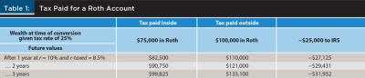
The moment the conversion occurs, both alternatives produce the same wealth: $75,000 net. But once compounding begins, the alternative of paying tax outside pulls ahead.

The outside branch has two components: the visible $100,000 in the Roth account, and the invisible, but very real, future value of the $25,000 sent to the IRS. Had it not been paid out in tax, this $25,000 could also have been invested in stocks earning 10 percent but tax would be due on earnings. It is convenient in this initial analysis to assume that the total gain would have been taxed each year at 15 percent. The compounding rate r-taxed is therefore approximated by 8.5 percent, calculated as (10 percent × [1 – 0.15]).

After three years, the Roth with tax paid inside is worth $99,825. The Roth with tax paid outside is worth $133,100 minus the future value of the funds sent to the IRS (–$31,932), or $101,168 in total. Paying tax outside created extra wealth of $1,343.

The dollar amount of the advantage gained from paying tax outside scales exponentially over time. A $1,343 advantage after three years becomes an $8,319 advantage after 10 years and a $40,386 advantage after 20 years.

It follows that any evaluation of a Roth conversion must be specific about the time span that will elapse before outcomes are evaluated. The longer the time frame—and 20 years is not that long for retirement income planning—the greater the dollar payoff is likely to be.

  Equation 2: 

      [(1 – tax ’) × $X] × (1 + r)^N < $X × (1 + r ’)^N

                            for 1 < N < k, and

      [(1 – tax ’) × $X] × (1 + r)^N’ > $X × (1 + r ’)^{N ’}

                                   for N ’ ≥ k

In words: if an additional tax payment must first be made to obtain the amount needed to pay conversion tax outside, the conversion will show a loss for k years, until compounding catches up.

Explanation. Planners are taught that compound interest must produce a greater accumulation than simple interest; in terms of arithmetic, over more than one time period (1 + i)^t > (1 + [i × t]). For example, on a five-year certificate with annual interest at 10 percent, simple interest on an investment of $100 will produce $150, while compound interest produces $161.05.

This simple inequality clears the way for breakeven analyses. Consider the saver who had only $95 to invest in that certificate, after paying taxes and fees to free up the funds. With compound interest over five years, that saver will still do better than the saver who had the full $100 to invest but only at simple interest: $153 versus $150. But this would not be true for a four-year certificate: $139.09 versus $140.

Let k be the number of years required to break even when a reduced amount is invested at a higher rate of return. No matter how great the reduction in amount, there will be some number of years k where breakeven will be achieved. In the running example, if only $80 is available to invest after taxes, compound interest on it will exceed simple interest on $100 after 10 years.

Equation 2 formalizes this insight within the context of paying tax outside the conversion but having also to pay additional tax to free up the funds used to pay that conversion tax. However, the idea of a breakeven point is more general; later we will introduce an entire class of Roth conversions that initially lose money, but still do eventually pay off.

Practical implication. In many cases, there will not be $25,000 in funds available with a 100 percent fraction of cost basis. Rather, because these funds had been invested years ago, there will be an unrealized capital gain. At the extreme, funds in the taxable account earmarked to pay conversion tax might be all capital gain, with 0 percent cost basis. In that case, if a long-term capital gains rate of 15 percent applies, the client will need to liquidate $29,411 in order to have $25,000 to send to the IRS to pay tax on the conversion proper. The Roth account, net of paying everything needed to pay tax outside the conversion, starts out with a $4,411 deficit relative to paying tax inside. Equation 2 indicates that this arithmetic difference can be overcome in time because compounding must overcome any non-compounded difference.

The question is, how long will it take for compounding to work its magic? This depends on the after-tax return that could have been earned on the outside funds if they had not been liquidated to pay conversion tax. The $4,411 deficit will melt away eventually, but the planner needs a good grasp on how long this will take before recommending a conversion that requires the client to pay tax in two stages.

Thus far we have been using a mark-to-market approach in which 15 percent capital gains tax is paid annually on all gains, making r-taxed 8.5 percent. At the other extreme, if an asset is held until death, there will be a step-up on any unrealized gain and only annual dividends will be taxed. If qualified dividends are 2 percent of the 10 percent total return before tax, then only 30 basis points would be lost to tax each year, and r-taxed becomes 9.7 percent. In between, we may have a more affluent client, one subject to a 20 percent rate on qualified dividends, and subject to net investment income tax (NIIT), thus paying a rate of 23.8 percent. Let this client also be one who prefers dividend-paying stocks, and who expects 4 percent of their total 10 percent return on equities to come from qualified dividends. If held until death, this client gives up 0.04 × 0.238, or 95.2 basis points in tax each year, and their r-taxed is 9.05 percent.

Figure 1 charts the breakeven time for these three cases. It shows breakeven points of 12, 19, and 60 years for r-taxed of 8.5 percent, 9.05 percent, and 9.70 percent. Put another way, it can take a long time to break even when tax has to first be paid to liquidate the funds needed to pay conversion tax outside the conversion. Planners need to recognize this reality; yes, it is optimal to pay tax outside the conversion if the client has funds with a 100 percent cost basis available. But in the case of large conversions, it will be a rare client who has tens of thousands of dollars in a bank account, ready to be liquidated without incurring any tax. In most cases, outside of a windfall, their adviser would have helped them to invest those funds years ago.

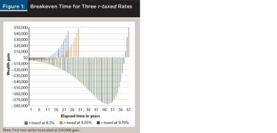
The time span of evaluation again emerges as critical. A client who had only a 10-year horizon could reasonably reject the strategy of paying tax from outside the conversion in cases where thousands of dollars in tax had to first be paid to obtain the outside funds with which to pay the conversion tax proper.

Paying tax outside the conversion will always eventually break even. But if the breakeven point falls outside the client’s planning horizon—or life expectancy—it is probably better to pay tax from inside the conversion. The older the client—or the sooner a step-up in basis may be expected—the stronger the argument for not incurring additional tax to get the funds needed to pay conversion tax outside.

Optimal time to convert. Because the benefit of paying tax outside the conversion scales exponentially with time, the optimum time to convert (with tax paid outside in cash) is earlier rather than later. A conversion undertaken at age 60 will have 12 extra years of compounding relative to one undertaken at age 72.

Optimal motive for conversion. Funds intended to be passed to heirs are an ideal candidate for conversion. Under the SECURE Act of 2019, final distribution of the TDA occurs over 10 years beyond the life span of self and any eligible designated beneficiary, giving compounding that much more time to magnify the payoff and/or to break even.³ DiLellio and Kinsman (2020) estimated this to generate an additional 13 percent of value for the heir (see also Young 2020).

De Minimis Rule

Consider a client with 100 percent cost basis funds in a taxable account and a 10-year planning horizon. With r-taxed of 9.70 percent, the dollar advantage for paying tax outside the $100,000 conversion produces an extra wealth gain on the conversion of 1.75 percent after 10 years—rather less than in the initial example where a 15 percent tax was marked to market each year.

Such a client can rationally argue that the incentive is not great enough; the advantage of retaining $25,000 outside of any tax shelter, with complete liquidity, outweighs the de minimis wealth gain from liquidating those funds to bulk up the Roth. Another equally rational client could say that a 10-year gain of well over $1,000 is more than enough to motivate paying tax outside a $100,000 conversion.

The arithmetic will always favor paying conversion tax outside if the time span is long enough. But the client is not bound to follow any narrowly calculated arithmetic advantage; the more so when the expected gain shrinks toward zero in percentage terms.

In practical life, the decision that some benefit is de minimis is a judgment call, and this judgment can only be made by the client. Planners should not recommend a Roth action without first calculating the dollar payoff over the time horizon that concerns that client and ascertaining whether the client judges the benefit to be sufficient.

  Equation 3: 

  k × X = X × k

This equation has ruled Roth conversion planning from the beginning. Its application will become more clear by substituting (1 – tax) for k and (1 + r)^N for X, and interpreting placement before and after as placement in time.

  (1 – tax₁) × (1 + r)^N = (1 + r)^N × (1 – tax₂)

  for 0 < tax₁ < 1 and tax₁ = tax₂

In words: paying tax on income up front and investing the remainder in a tax-free account (Roth case) must produce the same final wealth as placing the full amount of income in a tax-deferred account and then paying that same rate of tax on its withdrawal (traditional case).

The equation only holds, of course, if tax_CONV = tax_DIST, and if r and N have the same value in both expressions. With those conditions, the outcome is guaranteed by the commutative property of multiplication.

Practical implication. If the tax rate at conversion is the same as the tax rate at withdrawal, the client is indifferent toward conversion. There’s no gain or loss to be expected from converting because, unlike the previous examples, the conversion tax is paid from the IRA assets.⁴ Tax has to be paid at some point, either at conversion or when unconverted amounts are withdrawn. The timing has no effect on after-tax wealth.

If tax_CONV is less than tax_DIST —if the tax rate to convert is less than the tax that would later have been due on withdrawal—then conversion is advantageous; if the reverse, then the conversion is not a rational choice and should not be undertaken.

That, at least, is the conventional wisdom.

Equation 3 Reworked

Equation 3, although appealingly simple in the formulation k × X = X × k, is inapt for the typical conversion situation. As expressed, one conversion occurs and then one distribution is made—i.e., a lump sum withdrawal. The first assumption is acceptable, but the second assumption runs counter to the practical situation that many conversions are designed to address.

By definition, a traditional tax-deferred account is subject to required minimum distributions. No lump sum withdrawal is ever required prior to death. Therefore, one desirable effect of a partial conversion may be to reduce future RMDs.

If tax_DIST for each RMD always equals tax_CONV, then Equation 3 easily generalizes from the two-period case to the multiyear case where RMDs are taken rather than a lump sum withdrawal. Here it is the distributional property of multiplication that guarantees the result.  

  Equation 3a:

In words: if the tax rate stays constant, then it doesn’t matter if the distributions occur as a lump sum or are split into multiple distributions.

Numerical example. Introducing RMDs and moving to a multiyear analysis makes it difficult to intuit whether the equality asserted in Equation 3a holds. A spreadsheet enumeration will show that it does. In this setup there are two groups of entries: the wealth accumulated by the $100,000 Roth conversion (with tax paid inside for simplicity), and the wealth that would have been accumulated under the counterfactual, in which no conversion occurs and the entire $100,000 remains in the tax-deferred account.

Because the counterfactual throws off RMD income, a corresponding distribution must be made each year from the Roth to maintain equivalence. If this was not done, the counterfactual would be generating consumption wealth not captured in the spreadsheet, which only shows financial wealth. The Roth distribution is made to correspond by multiplying the dollar amount of the counterfactual RMD by (1 – tax_DIST).

To further simplify the illustration, assume the conversion is made just before the end of the year the couple turns 72.⁵ The conversion of $100,000 thus reduces the first RMD due next year at age 73 and produces tax savings if any from that point.

Wealth accumulation is evaluated each year by comparing the Roth account value to the counterfactual TDA balance multiplied by (1 – tax_DIST). Table 2 maintains a constant tax rate throughout, i.e., tax_CONV = tax_DIST. The expected outcome per the arithmetic is that the conversion has no wealth impact: after-tax wealth in the two accounts will be the same at every point. Later tables in this paper will raise and lower the distribution tax rate to calibrate the dollar amount of the conversion benefit (cost) when the tax rate does change between conversion and the onset of RMDs.

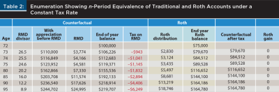
Table 2 works out the results for a constant tax rate of 25 percent. At conversion there is $75,000 in the Roth after paying the conversion tax from inside.

1. At the end of period 1, the counterfactual has appreciated to $110,000, from which the first RMD of $3,774 is taken,⁶ leaving $106,226, all of which will be subject to tax at some point. Its after-tax value at that point is $79,670.
2. The Roth account has appreciated to $82,500, from which a corresponding distribution of [$3,774 × (1 – 0.25)] = $2,830 is deducted, leaving $79,670, identical to the after-tax value of the counterfactual.

In subsequent periods, the dollar amounts increase, but the two accounts again produce the same after-tax wealth. The enumeration given in Table 2 confirms the equality in Equation 3a.

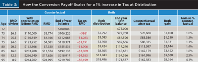
Next, Table 3 is structured the same, but the tax rate is made to differ. Here RMDs are subject to a tax_DIST that is 1 percent higher than the tax_CONV rate. Now there is a first-year payoff to the Roth conversion of $1,100. The payoff scales with time at the rate of return on the Roth account (10 percent), growing to $1,210 after two years and $1,331 after three. Unsurprisingly, the first-year payoff from avoiding a 1 percent future tax hike equals 1 percent of the counterfactual balance before RMDs. Over time, as RMDs slow the growth in the counterfactual balance, the projected conversion payoff grows to be 1.8 percent of the remaining balance by age 85 and 4.1 percent by age 95 (right column).

The interested reader can download the spreadsheet from the authors’ website to satisfy themselves that the following statements hold:⁷

1. The dollar payoff scales arithmetically with the percentage point increase in future tax rates. First year conversion payoff for a 2 percent rate hike will be $2,200 and for a 3 percent hike $3,300. Later ages will maintain that ratio, i.e., later values for a 2 percent or 3 percent hike will also be two times or three times those for a 1 percent hike.
2. If the conversion was ill-timed and future tax rates go down, the payoff will be the exact negative, with a loss of $1,100 after one year for a 1 percent tax cut, –$2,200 for a 2 percent cut, and so forth.
3. If the rate of return on account assets is lowered to 5 percent, the payoff in the first year will drop to $1,050 because the counterfactual only grew to $105,000 at that lower rate of return. Second year payoff will be only $1,102.50, not $1,210. With each year, the dollar payoff from conversion will fall exponentially further behind the base case of an asset returning 10 percent.

Practical implication. There are a few takeaways from this.

1. The steeper the future tax hike, the greater the dollar payoff from a conversion.
2. But for any given increase in tax_DIST, the greatest dollar payoff from a Roth conversion occurs when high return assets are converted, e.g., stocks rather than bonds or balanced funds.⁸ 
3. Longer time horizons magnify the dollar amount of whatever payoff is received.

Death and Infirmity

Death tends to drive tax_DIST higher, either rescuing what had been a misbegotten conversion or leveraging a successful one. Death enters the arithmetic in two ways. For most couples, one spouse will outlive the other by some years. RMDs for the survivor will be taxed at the single rate, which will almost always be higher than the couple’s rate, even after possible reductions in income due to loss of a portion of Social Security. The payoff boost from widowing will tend to increase with the gap in years between the first and second death and decrease the later the year of the first death, with the total conversion payoff a function of the blend of tax_DIST rates applied.

Second, under the SECURE Act of 2019, retirement balances must generally be distributed within 10 years of death.⁹  The RMD divisor becomes 10.0 for those years, a level that the living would not reach until age 94. Larger distributions may push the heirs into higher tax brackets, or the heirs may be in the prime of their career and already in a higher tax bracket than the retirees (Young 2020).

Infirmity tends to cut the other way, reducing tax_DIST. Late in life, large withdrawals beyond the minimum may be required to support assisted living expenses or to cover illness (Blanchett 2014). Under current law, these withdrawals may be deductible all or in part as medical expenses. That drives tax_DIST toward zero for those withdrawals.¹⁰ Conversion payoffs may prove de minimis in the final tally.

Practical implication. The further out the spreadsheet projection runs, the more uncertain the calculation of conversion payoffs must be (Harvey 1993). A conversion whose calculations do not show a large payoff until the client’s 90s may not pay off by much at all.

Inasmuch as an age of 90 will typically not be reached until 20 or 30 years after the conversion occurs, the careful planner will communicate to clients the present value of the expected payoff, or at least express it in constant dollars. Sophisticated clients may request best case / worst case projections in addition to the base case. A widowing analysis plus a high assumed tax rate for heirs can show the greatest payoff to be reasonably expected, and N years of assisted living expenses can peg the worst reasonable outcome.

  Equation 4: 

   If A < B (Equation 1) and

   u = v (Equation 2), then                 

   A + u < B + v

This equation allows a challenge to conventional wisdom about Roth conversions. The arithmetic will show that a Roth conversion can pay off even when tax_DIST is equal to tax_CONV; in fact, most Roth conversions will pay off, even when tax_DIST is lower than tax_CONV. The question for clients will be whether the breakeven time is acceptable and whether the payoff is judged more than de minimis.

The previous section argued that given RMDs, a proper comparison required that Roth distributions also be taken, with the amount matched to the after-tax amount of the counterfactual RMD. Although theoretically correct, this arrangement cuts against common practice. A frequent motivation for conversions is precisely to place funds where they can be invested for the very long term without being subject to withdrawals.

An equally proper comparison can be obtained if two changes to the spreadsheet model are made. First, take no distributions from the Roth; but second, reinvest the after-tax portion of each counterfactual RMD in an ordinary taxable account. This decision does not violate ordinary practice. To fund a Roth conversion in order to reduce distributions implies that these funds are not needed for consumption. If the funds are not needed for living expenses, then after paying the IRS its due, the remainder of the counterfactual RMD can be reinvested in the same asset(s) as before.

The effect of reinvesting after-tax RMDs is to split the counterfactual no-conversion account into two pieces: one a tax-deferred account, subject to Equation 3 when compared to a Roth, and the other a taxable account, subject to Equation 1 when it is compared to the corresponding portion of the Roth. Equation 4 guarantees that when the two pieces of the counterfactual are added together and compared to the Roth, and when enough time is allowed to pass, after-tax wealth in the Roth must be greater, even when tax_DIST equals tax_CONV.

The discussion of Equation 1 showed that the Roth advantage over a taxable account will scale exponentially with time. That fact enabled breakeven analyses, as in the example of compound versus simple interest. The same logic will show that Roth conversions always pay off, in time, even when tax_DIST comes in lower than tax_CONV. Once again, the length of the client’s planning horizon becomes crucial.

Numerical demonstration. The spreadsheet model from the previous section can be adapted by adding a third group of columns tracking the reinvestment of RMDs while removing the column showing Roth distributions. Table 4 gives the results for a constant ordinary tax rate of 25 percent with the assumption that the annual gain in the taxable account is all taxed at 15 percent. This mark-to-market approach simplifies the initial analysis since the reinvested RMDs will always have a 100 percent cost basis. A later analysis will use more realistic assumptions in which only dividends are taxed each year and cost basis is tracked (Roth 2020).

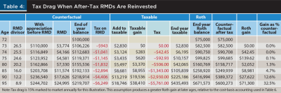
The metric again is the incremental after-tax wealth created by the conversion. The Roth value is compared to the taxable account (with its 100 percent cost basis) plus the after-tax value of the undistributed TDA portion of the counterfactual. In this first iteration tax_CONV = tax_DIST.

1. After one year there is no gain from the conversion. That’s because the first RMD has not yet been invested—the taxable account has only just been created from the RMD. Therefore Equation 3 applies, and the after-tax wealth is the same because the tax rate at distribution is the same as the tax rate at conversion.
2. In year two, a conversion payoff appears. It is equal to the tax assessed on earnings from the invested portion of the first RMD, $42.45. Those funds have been lost to the client, paid out to the IRS and gone. The dollar payoff for the Roth conversion is quite small at this point, about four basis points of the $100,000 conversion. The first RMD was only 3.77 percent of the counterfactual; only 75 percent of it was available to be invested; it earned 10 percent; and only 15 percent of that 10 percent was lost to tax to the advantage of the Roth.
3. In year three, the wealth gain is greater, at $139.62. Two RMDs have been reinvested, one for two years, and the second larger than the first. But, and this is central to the analysis, $139.62 is not equal to the sum of the tax burden paid in years two and three. The two tax payments together add up to only $135.38. The wealth gain is $4.24 greater. And that value of $4.24, of course, is the result of compounding the first year’s tax drag at the asset return rate (10 percent). Tax drag compounds because the $42.45 lost in tax on the taxable account was not lost to the Roth; it stays there and continues to appreciate.
4. As the years pass, the incremental wealth gain rises faster and faster as new tax drag gets added and prior tax drag compounds further. The taxable portion of the counterfactual falls further and further behind the corresponding portion of the Roth, per Equation 1.
5. By age 85, the percent gain on the conversion (right column) from tax drag at constant tax rates notably exceeds the gain from a simple arithmetic difference of 1 percent in the tax_DIST rate (compare right column of Table 3). Tax drag compounds. Compounding is an exponential process.

Practical implication. Roth conversions are robust against mistaken assumptions about tax_DIST but only over the long run. Tax drag starts very small and mounts slowly over the first decade. Large payoffs will require decades if tax_DIST is not higher than tax_CONV.

Breakeven Analyses

For these breakeven analyses it is no longer appropriate to assume a 15 percent capital gains tax marked to market each year. Instead, for the base and most likely case, placed in the second column of Table 5, the stock return of 10 percent is split into 2 percent dividend payments and 8 percent unrealized gains. Dividends are taxed each year, but the unrealized gains are allowed to compound. When evaluated annually, the value of the taxable account portion of the counterfactual is the stated accumulation, minus the cost basis to that point, multiplied by (1 – tax), with tax equal to 15 percent. This parallels how the tax-deferred portion of the counterfactual is treated.

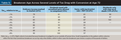
Next, more affluent clients will pay a long-term gains rate of 20 percent plus 3.8 percent NIIT. This will produce greater tax drag, and the third column in Table 5 shows the impact.

The left and right columns of Table 5 introduce more extreme cases to put some bounds on the breakeven analysis. The earlier discussion of Equation 2 showed that breakeven points are very sensitive to the magnitude of tax drag, i.e., the gap between r-taxed and tax-free r. Parallel to that discussion, the right column of Table 5 taxes dividends annually at 15 percent but assumes a step-up in basis at death for any unrealized gains, so that these never get taxed, making r-taxed approximately 9.70 percent, and reducing tax drag to a very small amount.

The left column examines the opposite extreme. There are strategies with equity-like returns where most of the annual return is subject to tax and at ordinary income tax rates. This could be a covered-call strategy, a high-yield bond fund, a REIT, a hedge fund, or any other strategy where ordinary income, non-qualified dividends, or short-term gains predominate. In between would be balanced funds where part of the income is ordinary interest. The extreme case here is thus an r-taxed of 7.5 percent (ordinary income tax of 25 percent marked to market every year).

Taking the second column of Table 5 first, consider a client who made a Roth conversion in 2016 while in the 25 percent tax bracket. If real income in retirement stayed constant, these retirees now find themselves in the 22 percent tax bracket post-TCJA. Per the earlier discussion, after one year they will have a wealth loss on the conversion of 3 × –$1,100 = –$3,300. But if they follow the strategy of reinvesting the after-tax RMD, in the second year the conversion will begin to benefit from tax drag.

This conversion, with its unfavorable tax_DIST delta of three percentage points, will break even 16 years later at age 88. If the tax_DIST delta had been negative four points (i.e., conversion at 28 percent, RMDs at 24 percent), breakeven would have been age 91. But a delta of eight points would not break even until age 100.¹¹

IRS mortality tables give insight into whether these breakeven points occur within human time.¹² A married couple, one of whom is age 73 and the other age 68, have a joint life expectancy of about 23 years, out to age 95 for a conversion at age 72, the year before RMDs currently begin under the SECURE 2.0 Act.

Practical implication. Many, perhaps most, Roth conversions can be expected to pay off within the joint life expectancy of a married couple, even when tax_DIST < tax_CONV. The tax on distributions has to come in six percentage points or more below the tax rate paid on the conversion to fail this test.

There is one other important exception. It pertains to conversion planning by individuals who do not have access to financial advice. These individuals may not grasp that tax brackets adjust annually for inflation, and thus miss the fact that income decades hence must be much higher in nominal dollar terms even to stay in the same tax bracket.

These individuals are at risk of converting at 22 percent to avert tax on RMDs that would fall into the next bracket lower and be taxed at 12 percent. That’s an unfavorable future tax delta of negative 10 percentage points. Even worse, long-term capital gains and qualified dividends are taxed at zero when income falls into the 12 percent bracket. Tax drag cannot occur prior to widowing, hence there is little prospect of breaking even.

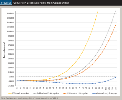
Understanding variations in tax drag. The assumed tax drag in the breakeven analysis thus far (Table 5, second column) has staked out a middle ground. It is possible today to hold a total stock market index ETF and pay taxes only on dividends and only at the 15 percent rate, with unrealized gains ultimately taxed also at 15 percent when realized. This reflects the situation of couples with adjusted gross income between about $100,000 and $500,000, or a broad cross-section of the mass affluent. But there are other scenarios, both more and less favorable to conversions, as shown in the other columns of Table 5 and graphically summarized in Figure 2.

Consider first the situation of a more affluent couple whose dividends and long-term gains will be taxed at 23.8 percent, a rate almost two-thirds higher (Table 5, third column). Interestingly, increased tax drag at this level provides only a modest improvement in breakeven age and mostly for larger deltas in tax_DIST.

Consider next the extreme cases in the left and right columns of Table 5. The results are asymmetric. Greater tax drag (r-taxed = 7.5 percent as opposed to a tax-free 10 percent) moderately accelerates breakeven time. An unfavorable tax_DIST delta of three points (25 percent → 22 percent) breaks even at age 83, not 88. But a lesser tax drag (r-taxed = 9.70 percent) causes breakeven ages to blow out. In the three-point case, breakeven stretches to an age of 103. Even a one-point delta in tax_DIST can’t be overcome until age 90, 18 years after conversion.

Figure 2 displays the characteristic curve shapes to be expected when breakeven occurs through compounding. With an unfavorable tax delta of minus three points, even in the best case, it takes over a decade to break even. Conversely, given enough time, breakeven does eventually occur within human time, even for more unfavorable tax_DIST deltas up to six points, excepting the extreme case where tax drag is minimal.

Practical implication. If the client has the discipline to reinvest RMDs into a passive stock index fund with the expectation that these will be held until death, tax drag will be so small and slow as to provide little protection for the conversion against adverse changes in tax_DIST (e.g., future tax cuts). However, given the same discipline, but uncertainty about whether invested RMDs may have to be tapped while alive, such a client can have some confidence that moderately adverse movements in tax_DIST may be overcome within joint life expectancy (Table 5, second column).

If the client will invest in anything other than a passive index fund with a dividend yield on the order of 2 percent—or if the client pays more than 15 percent on annual earnings in the taxable account—then tax drag provides good protection against adverse changes in tax_DIST. A case in point: California taxes long-term gains and qualified dividends as ordinary income. The affluent middle-class Californian can expect tax drag on these of 15 percent + 9.3 percent = 24.3 percent, raising the protective character of tax drag to the levels seen in the third column of Table 5.

De Minimis Rules Revisited

To know that a Roth conversion will probably break even is reassuring; but arguably, most retirees contemplating a conversion hope to see a substantial wealth gain. This section calibrates the wealth gain to be expected from a conversion with a moderately favorable or unfavorable movement in tax_DIST across the base case for expected tax drag (Table 5, second column). Conversion payoff is evaluated at age 85, 90, and 95 for conversion at age 72. In addition to nominal dollar amounts, constant dollar amounts assuming inflation at 3 percent are given as a percent of the $100,000 conversion.

Consider first the 0 percent row in the middle of Table 6, with tax_CONV always equal to tax_DIST. Any gain here is pure tax drag. The payoff grows to be quite substantial at the later ages. In fact, adding a favorable tax_DIST delta provides what might be called only incremental gains over what tax drag alone contributes. This is most clearly seen by examining the percentages, which show real dollar gain as a percent of the $100,000 conversion. At age 95, tax drag alone under constant rates produces a real gain of 25.6 percent. Each one percent movement up in tax_DIST (lower rows) adds only about 4.2 percentage points of additional gain.

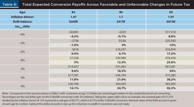
At somewhat younger ages such as 85, the pattern is different. The payoff from tax drag alone is still substantial, but the contribution of a favorable movement in tax_DIST is greater. This follows directly from Equations 1 and 2: tax drag scales exponentially with time. The less time elapsed, the less the ability of tax drag to overcome the arithmetic difference from an unfavorable movement in tax_DIST, per the breakeven analyses above. Tax drag compounds, but compounding takes time to produce really large amounts.

Practical implication. The ideal client for a Roth conversion has a time horizon that extends into their mid-90s or beyond. For that client, tax drag should be potent enough to overcome any moderately unfavorable movement in future tax rates. Even for an unchanged tax_DIST, their conversion would still produce tens of thousands in real dollar gain at the end of their planning horizon.

By contrast, a client who does not expect longevity and who is confident that funds will be unneeded before death is a poor candidate for conversion. Given a step-up in basis, tax drag is too small to overcome almost any unfavorable movement in future tax rates at any age before the 90s. Only a favorable movement in future tax rates can make a Roth conversion pay off for such clients. For them, the conventional wisdom is largely correct: do not convert now, absent a conviction that future tax rates will move higher (and stay higher).

Alternatively, if client and adviser do not feel much confidence in their forecast of future tax rates, the decision rule for clients with a short horizon defaults to the question of whether conversion tax can be paid from outside funds with a 100 percent cost basis—and as early as practicable. As shown in the discussion of Equation 1, tax paid outside and early builds in additional gains on the conversion. With tax paid outside there is additional tax drag, with one source beginning to compound years earlier. That doubly boosted conversion should be robust even at younger ages.

The Riskiest and Least Robust Conversions

There are three kinds. The first has already been discussed: conversion low in the 22 percent bracket while neglectful of the inflation adjustment applied annually to tax brackets, leading to RMDs taxed at 12 percent and no tax drag because no tax on dividends and long-term gains. The post-TCJA scheduled rise in rate to 15 percent will not rescue this conversion.

The second is when the TDA funds may ultimately be donated to a charitable organization that receives pre-tax assets but, absent a tax law change, will owe no taxes on the charitable gift.

The third disaster scenario may surprise some advisers: conversion while in a top tax bracket. Two factors combine to produce this result. The first is common sense, not arithmetic: the higher the tax rate paid to convert, the greater the opportunity for the rate applied to distributions to move substantially lower, either because tax cut legislation is passed or because the converter’s future income falls short of expectations, leading to RMDs taxed in a lower bracket.¹³ The second reason does come down to arithmetic, as a concrete example will make clear.

Consider a resident of California or other high-tax state. If their income is above $700,000, the current combined federal and state rate will be about 48 percent. Their tax_DIST rate could of course move higher still: if TCJA rates lapse as scheduled, their rate will go to 50.6 percent. But if the conversion occurs a dozen years before RMDs begin, and inflation runs at 3 percent, they will need retirement income in excess of $1 million to have the last dollar taxed at that 50.6 percent. If the goal of the conversion(s) was to reduce RMD income by $50,000, they will need to project $1,050,000 of inflated future income for the 50.6 percent rate to apply to the entire reduction. If their income falls short of that level, they will drop one federal bracket and one California bracket. The conversion will have averted tax on RMDs at 45 percent, a three-point drop in tax_DIST.¹⁴ 

Here is where arithmetic enters the picture. The third column of Table 5, showing the top long-term gains rate that would apply to this couple, shows breakeven age for a tax_DIST delta of negative three points as 87. But when tax_CONV is 48 percent, not the 25 percent assumed in Table 5, the breakeven age stretches to 90. The reason: when 45 percent of the RMD goes to tax, the dollar amount placed in the taxable account is smaller than when only 22 percent of it went to pay tax. Dollars paid for tax on the earnings in that smaller account are reduced accordingly. Tax drag starts smaller, hence takes longer to overcome the unfavorable tax_DIST delta.

The stretch out in breakeven age becomes more dramatic at more unfavorable tax_DIST deltas. The 10 percent bracket in California is quite narrow; a slightly greater income shortfall would put the retirees in the 44 percent bracket. In Table 5, the breakeven age for that delta of minus four percentage points was 89; with a tax_CONV rate of 48 percent it is pushed out to 93. At the extreme, the converters retire to Nevada or Washington, eliminating state tax and producing a negative delta of 13 points. Per Equation 2, their conversion will nonetheless ultimately break even . . . at age 114.

Practical implication. A robust conversion is one that can succeed under a wide range of favorable and not so favorable future developments, with success measured in terms of wealth gain received within the client’s planning horizon. Conversions by residents of high-tax states, particularly those with income subject to the top federal brackets, are not as robust.

Conversions near the floor of a bracket located above a gap in the bracket structure (current rates of 32 percent or 22 percent) are also not robust; there are too many possibilities whereby RMD income could get taxed in the next bracket down at a steep decline in tax rate. Conversions low in the current 22 percent bracket are particularly fraught so long as the bracket below retains a qualified dividend tax rate of zero.

Conversions where the future tax rate might be close to zero are likely to fail. This includes funds that would have gone to charitable organizations, but also funds that might be inherited by grandchildren or other minor heirs, or by any very low-income heir.

There appear to be two sweet spots in the current tax structure (apart from conversion at an initial tax rate of zero). Couples whose conversions occur high in the current 12 percent bracket face few prospects of RMDs being taxed at a significantly lower rate. Their situation is the inverse of those in the top brackets.

Second, conversions in the current 24 percent bracket, if undertaken before age 63 and thus not likely to trigger Medicare income-related monthly adjustment amounts (IRMAA) due to income from two years prior (Pfau 2021), will generally be robust. Retirement income would have to drop $100,000 or more short of projections, even to fall out of the minimally lower 22 percent bracket, which in any case is scheduled to rise to 25 percent post-TCJA. Retirement income throughout the 24 percent bracket will also generally be subject to IRMAA, adding 4–5 percent to whatever future income tax rate applies, and almost ensuring a positive tax_DIST delta. Conversions in this federal bracket by residents of states with no income tax, such as Washington, Texas, and Florida, are particularly robust.

Limitations

The primary limitation is the restriction to advice that could be supported by simple arithmetic. The optimal deployment of Roth accounts permits much more sophisticated mathematical analysis (e.g., DiLellio and Ostrov 2020).

Future research needs to address the fact that tax_DIST is not a scalar quantity as assumed in the arithmetic. Tax_DIST is more like a quantum particle: at the time of conversion, it exists only as a probability distribution, a vector of future rates whose entries can change at any point. This uncertainty makes Roth payoff estimates fallible. Whatever value of tax_DIST was expected, the realized tax rate may come in lower, causing a loss on the conversion until tax drag makes it up. Alternatively, over longer retirements, the value of tax_DIST is unlikely to stay the same. That can boost conversion outcomes, as when a widowed survivor must pay a higher tax rate; or it can delay payoffs if temporary tax cuts are legislated. More sophisticated mathematics will be required to quantify the odds that the conversion payoff will be positive and exceed the client’s threshold for de minimis outcomes.

There is more uncertainty. IRMAA will serve as a stand-in for the class of “supplemental taxes added on to income tax,” a class that also includes what Reichenstein and Meyer (2020) describe as the Social Security tax torpedo. IRMAA and its kin tend to raise the total effective tax_DIST (see also Pfau 2021). To some extent, IRMAA is a penalty on prosperity: most of the penalty is incurred in moving through the 24 percent income tax bracket, corresponding to AGI for couples of about $200,000 to $400,000 in 2023 dollars. IRMAA raises the marginal tax rate in this zone to at least 29 percent, making pre-IRMAA conversions at 24 percent or 22 percent a good wager, to the extent these reduce IRMAA charges after RMDs begin. On the other hand, if the conversion takes place in the 24 percent bracket within two years of enrollment in Medicare B, the conversion itself may incur IRMAA charges, making tax_CONV 29 percent, thus increasing the odds that tax_DIST comes in lower.

The paper also did not consider alterations to the tax code that are invidious to Roth accounts. For instance, today the MAGI used to determine IRMAA includes otherwise tax-free income from municipal bonds but excludes otherwise tax-free income from Roth distributions. That could change. The future is unknowable, and the future tax treatment of Roth accounts is no exception.

Future research might attempt to simulate many possible vectors of future tax rates (e.g., widowing early or late, with shorter or longer life for the survivor) in an effort to estimate the odds that conversion at a given tax rate, at a given age, will pay off over some time span. But that will require a more sophisticated mathematical treatment than anything attempted here.

Conclusion

On the arithmetic, conversions are a good bet for the mass affluent. But some clients will not have the patience to play, and others may not find the expected payoff enticing. 

Citation

McQuarrie, Edward F., and James A. DiLellio. 2023. “The Arithmetic of Roth Conversions.” Journal of Financial Planning 36 (05): 72–89.

Endnotes

1. The attribution of this quote to Albert Einstein has been judged apocryphal: https://quoteinvestigator.com/2011/05/13/einstein-simple/.
2. For simplicity, this paper will ignore the many special cases that depart from this simple description. For instance, a five-year rule applies to tapping funds from a converted IRA; accounts inherited by a spouse are subject to different RMD rules than for non-spouse heirs; and many more. In addition, trading costs are assumed to be zero throughout.
3. See Notice 2022-53, 2022-45 I.R.B. 437 (Oct. 7, 2022).
4. Assumes the individual converting the IRA is at least 59½ to avoid early withdrawal penalties.
5. The SECURE 2.0 Act legislation, passed in December 2022, raised the required beginning age to 73 until 2033, when it becomes 75. It did not change the RMD schedule introduced in 2020. See www.federalregister.gov/documents/2020/11/12/2020-24723/updated-life-expectancy-and-distribution-period-tables-used-for-purposes-of-determining-minimum.
6. The RMD amount is set by the previous year-end balance, $100,000 to start.
7. Available at www.edwardfmcquarrie.com.
8. This paper does not address the more complicated arithmetic that applies when a Roth conversion is used to alter asset location, i.e., to preferentially convert stock assets and leave the TDA more heavily allocated to bonds. See Reichenstein, Horan, and Jennings (2015).
9. See endnote 3 for the details of how the 10-year rule is interpreted.
10. Because medical expenses are only deductible over a threshold, tax on the distribution is unlikely ever to reach zero; but it may be considerably lower than the tax_DIST projected when planning the conversion.
11. Although we use the drop from 32 percent to 24 percent as a believable instance of an 8 percentage point drop under the current tax code, the values in the table all use a conversion tax rate of 25 percent for consistency, i.e., the breakeven for an eight-point drop is computed for a decrease in rate from 25 percent to 17 percent. The same delta—e.g., 8 percentage points—has a somewhat different effect when the tax_CONV rate is higher or lower. See discussion in a later section.
12. The IRS mortality tables can be found in the Federal Register; see endnote 5.
13. The rescue potential from widowing is also lower in the top brackets. Because of the articulation of single versus married brackets at the top of the rate structure, a couple taxed at 35 percent or 37 percent may produce a widowed survivor still taxed in those brackets and with a lower IRMAA burden as well.
14. In actuality, the TCJA adjusted bracket boundaries as well as rates, and those bracket adjustments will lapse as well if TCJA sunsets as scheduled. A larger drop in income than suggested in this illustrative paragraph might be required to drop one federal bracket in 2026.

References

Blanchett, D. 2014. “Exploring the Retirement Consumption Puzzle.” Journal of Financial Planning 27 (5): 34.

Brown, D.C., S. Cederburg, and M.S. O’Doherty. 2017. “Tax Uncertainty and Retirement Savings Diversification.” Journal of Financial Economics 126 (3): 689–712.

Crain, T. L., and J. R. Austin. 1997. “An Analysis of the Tradeoff Between Tax Deferred Earnings in IRAs and Preferential Capital Gains.” Financial Services Review 6 (4): 227–242.

Clayton, R., L. Clayton, L. Davis, and W. Fielding. 2014. “Converting to a Roth IRA with Taxes Paid from Corpus of the Traditional IRA.” Journal of Applied Finance 24 (1).

Coopersmith, L. and A.R. Sumutka. 2017. “The Impact of Rates of Return on Roth Conversion Decisions and Retiree Savings Wealth.” Journal of Personal Finance 16 (1).

DiLellio, J., and D. Ostrov. 2020. “Toward Constructing Tax Efficient Withdrawal Strategies for Retirees with Traditional 401(k)/IRAs, Roth 401(k)/IRAs, and Taxable Accounts.” Financial Services Review 28 (2): 356–384.

DiLellio, J., and M. Kinsman. 2020. “The SECURE Act and Your Retirement Objectives.” Graziadio Business Review 23 (2).

Harvey, A. C. 1993. “Time Series Models.” In Handbook of Statistics. MIT Press.

Horan, S. M., J. H. Peterson, and R. McLeod. 1997. “An Analysis of Nondeductible IRA Contributions and Roth IRA Conversions.” Financial Services Review 6 (4): 243–256.

Horan, S., and A.A. Zaman. 2013. “Risk-sharing Implications for Roth IRA Conversions: Fact and Fiction.” Financial Services Review 22 (2): 93–113.

Krishnan, V.S., and J. Cumbie. 2016. “Roth Conversion: An Analysis Using Breakeven Tax Rates, Breakeven Periods, and Random Returns.” Journal of Personal Finance 15 (1): 37.

McQuarrie, E. F. 2008. “Thinking About a Roth 401(k)? Think Again.” Journal of Financial Planning 21 (7): 39–48.

Mollberg, K.T., 2020. “Time to Consider a Roth Conversion: Maximize the Benefits of This Proven Strategy.” Journal of Accountancy 230 (4): 30.

Pfau, W., 2021. Retirement Planning Guidebook: Navigating the Important Decisions for Retirement Success. Retirement Researcher Media.

Reichenstein W., 2020. “Saving in Roth Accounts and Making Roth Conversions before Retirement in Today’s Low Tax Rates.” Journal of Financial Planning 33 (7): 40–43.

Reichenstein, W., S.M. Horan, and W.W. Jennings. 2015. “Two Key Concepts for Wealth Management and Beyond.” Financial Analysts Journal 71 (1): 70–77.

Reichenstein, W., and W. Meyer. 2020. “Using Roth Conversions to Add Value to Higher-Income Retirees’ Financial Portfolios.” Journal of Financial Planning 33 (2): 46–55.

Roth, A. 2020, September 14. “The Seven Cases to Do a Roth Conversion.” Advisor Perspectives. www.advisorperspectives.com/articles/2020/09/14/the-seven-cases-to-do-a-roth-conversion.

Young, R. 2020. “The Roth/Pretax Decision in Late Career Years: The Increasing Importance of Accumulated Assets in Light of the SECURE Act.” Journal of Financial Planning 33 (7): 59–68.