Safely Boosting Retirement Income by Harmonizing Drawdown Paths

Journal of Financial Planning: November 2020

 

Executive Summary:

• Building on Bengen’s famous 4 percent rule (Bengen 1994), this paper introduces the DMSWR, a technique for calculating withdrawal rates and retirement income levels that are safe, steady, and adjusted for inflation.
• The DMSWR (named after the authors’ initials, plus the acronym for safe withdrawal rate) addresses two commonly cited shortcomings of the 4 percent rule. First, it addresses the starting point paradox (Kitces 2008) by ensuring that initial retirement incomes are stable regardless of the precise retirement date and short-term fluctuations in the stock market. Second, the DMSWR significantly reduces the risk of unnecessarily low retirement income that leads to large, unspent portfolios at the end retirement.
• The DMSWR provides withdrawal rates that are often substantially higher, and never lower, than the 4 percent rule, which allows financial planners to recommend higher retirement incomes that are still safe.
• The core insight underpinning the DMSWR is that a retiree can safely follow the “drawdown path” of an earlier retiree who follows the 4 percent rule and planned for a longer retirement. Since the earlier retiree’s withdrawals are safe, the withdrawals of the new retiree must also be safe.
• The DMSWR is safe in the same way the 4 percent rule is safe: the withdrawal rates have never failed in the past and, were DMSWR to fail in the future, the 4 percent rule would also fail. Unlike many similar efforts to boost safe withdrawal rates, the DMSWR does not include additional parameters or heuristics that might fail at a time when following the 4 percent rule would succeed.
• Historically, the mean DMSWR for 30-year retirements was 5.48 percent, the highest DMSWR was 13.3 percent, and the DMSWR exceeded the baseline withdrawal rate by more than 100 basis points over 55 percent of the time.
• “Re-retirement” using the DMSWR often allows incomes to increase during retirement. These higher incomes succeed whenever the 4 percent rule succeeds.

David Marwood is a staff software engineer, working on the future of machine learning at Google. He completed his MSc at the University of British Columbia in 1996 and has a strong interest in both investing and retirement planning.

David Minnen is a senior research scientist at Google, where he works on machine learning methods for image and video compression. He received his Ph.D. at the Georgia Institute of Technology in 2008 where his research on unsupervised time series analysis was funded by an NSF Graduate Research Fellowship.

NOTE: PLEASE CLICK OR TAP FIGURES AND TABLES BELOW TO LAUNCH A PDF OF THE IMAGE. 

JOIN THE DISCUSSION: Discuss this article with fellow FPA Members through FPA's Knowledge Circles​​​​. ​​​

Clients approaching retirement often want to generate stable income from their retirement savings with minimal risk of early portfolio depletion. William Bengen was one of the first financial planners to address this problem in a principled way (Bengen 1994). He showed that a 50 percent stocks/50 percent bonds portfolio would supply an income of 4 percent of the initial portfolio value, indexed to inflation, for 30 years. This 4 percent value is “safe” in the sense that Bengen showed that it succeeded for all historical 30-year periods.

Bengen’s idea of a “safe withdrawal rate” (SWR) became the foundation of a large body of literature and is now colloquially known as the 4 percent rule. Bengen showed that different retirement durations and different asset allocations led to values other than 4 percent, and more recent researchers have also adjusted this number after analyzing more recent market data. To avoid confusion, the term “baseline SWR” will be used to describe Bengen’s general technique of calculating an SWR and pulling an inflation-adjusted income, regardless of the precise initial withdrawal percentage.¹

Kitces (2008) observed what he termed the starting point paradox of safe withdrawal rates. His work described two hypothetical clients, call them Alice and Bob, who have both saved $1 million for retirement. Alice wants to retire right now, and her financial planner recommends a 4.5 percent withdrawal rate yielding an income of $45,000 a year on her $1 million portfolio.

Bob decides to delay retirement for one year. Unfortunately, the following year sees a bear market in which both Alice’s and Bob’s portfolios decline 15 percent. At this point, Alice withdraws $46,350 based on her initial income of $45,000, adjusted for 3 percent inflation. For Bob, the financial planner again recommends a 4.5 percent SWR, which leads to an income of $38,250 a year based on Bob’s $850,000 portfolio. Despite starting with identical savings and retirement goals, Alice’s income is 21 percent higher than Bob’s, even though her current balance is lower than Bob’s due to her withdrawal in her first year of retirement.

This paper introduces the DMSWR, an approach for calculating safe withdrawal rates that resolves the starting point paradox. The core idea is based on the observation that if an existing retiree is drawing retirement income following Bengen’s strategy, a new retiree can always follow the same drawdown path, the series of withdrawal rates implied by the dollar withdrawals and corresponding portfolio values made during retirement, with no additional risk of early portfolio depletion. Since Bengen’s strategy calls for inflation-adjusted withdrawals, the existing retiree’s withdrawal rate as a fraction of their current portfolio value will fluctuate throughout retirement as the market and their portfolio value moves up and down. The rate will fall when the real-dollar portfolio value increases and the rate will rise when the portfolio value decreases. Crucially, a new retiree can follow the drawdown path of an existing retiree who currently has a high withdrawal rate, using the high withdrawal rate as their own, and be no less safe than the existing retiree.

The ability to follow another retiree’s drawdown path “harmonizes” the paths of different retirees. This removes the sensitivity of retirement income to the precise retirement date and insulates initial retirement incomes from short-term market fluctuations. The DMSWR uses this to resolve the starting point paradox. In the simple case where an existing and a new retiree have the same portfolio value, they will have the same withdrawal amount and the same portfolio value for their entire retirements. In addition, using the DMSWR rather than the baseline SWR often increases initial withdrawal rates since the new retiree can use the highest withdrawal rate of any existing retiree with the same retirement end date, mitigating concerns about large, unspent portfolios at the end of retirement.

In much the same way, a retiree in the middle of their retirement can choose to “re-retire” if they find a safe drawdown path that covers the remainder of their retirement but currently has a higher withdrawal rate. Re-retiring will thus lead to a boost in retirement income while maintaining safety against portfolio depletion, so long as the new drawdown path is safely following Bengen’s strategy.

In the worst case, the DMSWR will equal the baseline SWR but it never yields a lower retirement income, and in many cases, the DMSWR is much higher. In practice, this benefit often arises after a market decline when clients may be afraid to retire due to smaller portfolios. With the DMSWR, it becomes clear that financial planners have more flexibility than previously thought, and they can safely and responsibly recommend higher withdrawal rates than what is implied by the baseline SWR.

Literature Review

The primary goal of this work is to improve safe withdrawal rates in terms of providing retirement income that maximizes retiree’s standard of living while minimizing the risk of portfolio depletion. Toward this end, previous researchers have used heuristics and parameters to better describe historical and simulated data. Zolt’s (2013) target percentage adjustment, Klinger’s (2016) guardrails, Guyton and Klinger’s (2006) decision rules, and Kitces’ (2015) ratcheting rule all belong in this category. These techniques all risk overfitting, or explaining historical data using more parameters than the data can justify while failing to explain future data. This risk is particularly poignant for withdrawal rates that, like Bengen’s, claim to be 100 percent safe. If a heuristic improves outcomes for just a few extreme retirement dates (specifically, dates in 1929, 1937, and 1965-1966), then it will improve on the baseline SWR. However, it is not at all clear that such a heuristic will continue to work well in the future. Effectively, these techniques increase safe withdrawal rates by increasing the risk of overfitting. They can fail for some future sequence of returns, even when the baseline SWR continues to succeed. In contrast, the DMSWR avoids additional heuristics, parameters, or assumptions not already made by Bengen.

The second goal of this work is to address the starting point paradox, where the baseline SWR strategy leads to initial retirement incomes that can fluctuate substantially in response to short-term market movement. Kitces’ (2008) adaptive initial withdrawal rate subdivides the historical record based on price-to-earnings ratios (P/E) and calculates the SWR separately for retirements that begin when P/E ³ 20 and for those that begin when P/E < 20. Although effective to some extent, this approach has some limitations. First, P/E has transitioned over the threshold of 20 only rarely in history. While meaningful over long time periods, it rarely makes a difference to an individual retiree deciding to retire this year or the next. Second, initial incomes are still subject to the full volatility of the underlying portfolio, baring those rare threshold transitions. Third, this technique is subject to the same overfitting concern and can fail where the baseline SWR would succeed. In contrast, the DMSWR responds monthly to both small and large portfolio value changes to keep initial incomes steady, and it is guaranteed to be safe in the same way the baseline SWR is safe.

That said, the DMSWR is actually orthogonal and complementary to all the above techniques. Were a planner to see the advantages in these heuristics, they can readily be used in conjunction with DMSWR, realizing the benefits of both. The work presented here applies the DMSWR to Bengen’s technique because it is least vulnerable to overfitting and because it has traditionally set the standard for SWRs.

Some past works, such as Zolt (2013) and Klinger (2016), have explored methods that allow real income to decrease during retirement to improve SWRs. While it can be appealing to take a larger up-front income in trade for the risk of decreasing income in the future, that future decrease may be an unpalatable message for a financial planner to deliver and can decrease a retiree’s spending power at a time when they are least able to compensate. Exhibit 6.20 in Pfau (2017) offers a survey of the income reduction demands of several techniques. The DMSWR avoids this unpleasant possibility altogether.

Other works look at alternative income sources such as Social Security and various annuities (Pfau 2013) and apply SWRs to other countries (Pfau 2016). The DMSWR is fully compatible with and complementary to such efforts.

Zolt (2013), Klinger (2016), and Finke, Pfau, and Blanchett (2013) use Monte Carlo simulations. This allows more (synthetic) samples for modeling and can explore alternative, non-historical scenarios but risks transferring poorly to the real world, which may not be well-modeled by the simulation.

Finally, the Trinity study (Cooley, Hubbard, and Walz 1998) considered “safe” withdrawal rates that had a low probability of failure, rather than zero historical failures, in an effort to allow larger initial withdrawal rates. Zolt (2013) followed suit and ERN (2013) has continued this thinking. The DMSWR avoids this direction as a means of increasing SWRs specifically due to the increased chance of failure. There are already significant risks, even for methods with a 100 percent historical success rate, and the cost of failure is very high. Further increasing that risk seems imprudent and is not considered here.

A Tale of Two Clients

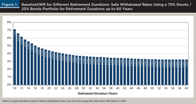
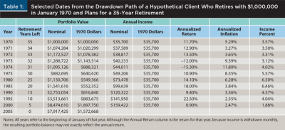
The DMSWR method addresses the starting point paradox by significantly reducing fluctuations in initial retirement income. Consider a hypothetical client named Carol. In 1970, Carol has saved $1 million in preparation for a 35-year retirement lasting through December 2004. Drawing from Figure 1, the Baseline SWR for Carol’s 35-year retirement allows for a 3.57 percent initial withdrawal rate, so her income starts at $35,700 per year and increases with inflation. Carol’s sequence of portfolio values and annual incomes, her drawdown path, are shown in Table 1.      

 

 

 

 

 

 

A different hypothetical client, Dave, would also like to retire in 1970, but Dave has not saved as aggressively as Carol and his portfolio value is too low to safely support $35,700 annual withdrawals. He, therefore, decides to continue working and saving for retirement.

Jump forward to the beginning of 1975. Carol is now withdrawing $49,206 per year (equivalent to $35,700 per year in 1970 dollars), and her portfolio has shrunk to $882,695 due to her withdrawals and adverse market conditions. After saving for five more years, Dave has accumulated, for illustrative purposes, $882,695 in his retirement account and, like Carol, his target income has increased to $49,206 a year due to inflation. Dave faces a planned retirement of 30 years, 1975 through 2004. Returning to Figure 1, the baseline SWR for 30 years is 3.69 percent, indicating that Dave can only safely withdraw $32,571 per year and, thus, according to the baseline SWR, Dave cannot safely withdraw his target income.

Dave and Carol have the same portfolio value, but the baseline SWR provides dramatically different safe income levels for them. Why can’t Dave follow Carol’s drawdown path starting in 1975? Dave is no less safe in withdrawing his target income of $49,206 per year from his $882,695 portfolio than Carol is. We know Carol’s withdrawals are safe and so Dave’s must be equally safe since the two retirees will withdraw the same amount, experience the same market conditions and, thus, see the same portfolio values for every month from 1975 through 2004.

A withdrawal of $49,206 on a portfolio value of $882,695 produces a current withdrawal rate for Carol of 5.57 percent, as shown in the Income Percent column of Table 1. If Dave follows Carol’s drawdown path, this 5.57 percent becomes Dave’s initial withdrawal rate for his 1975 retirement.

Table 1 starts with Carol’s retirement in 1970, but there is nothing special about that year. Dave can look back to any past year, keeping in mind that he can only follow retirements that extend at least as long as his own. Also, longer lookback periods result in decreasing initial SWRs, as shown in Figure 1. Due to the lower SWR and since portfolio values change month to month due to market movement, there is no guarantee that looking back further will result in a higher retirement income.

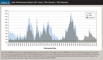
The DMSWR looks back at the historical data, searching for the best drawdown path to safely boost current SWRs. In general, the DMSWR says that a retiree can safely adopt the maximum current withdrawal rate of any previous retiree with the same final withdrawal date and portfolio composition, as long as the hypothetical retiree started with a safe withdrawal rate and follows Bengen’s withdrawal policy. In particular, a hypothetical January 1966 retiree with the same December 2004 final withdrawal date as Dave withdraws 3.48 percent in 1966 (39 years in Figure 1) and has a current withdrawal rate of 7.57 percent in January 1975. Dave can follow this drawdown path and use 7.57 percent as his initial withdrawal rate, which yields an income of $66,820 per year when applied to his $882,695 portfolio. This income is safe because the rate is safe for the 1966 retiree. Note that while Dave’s 7.57 percent withdrawal rate is safe for his January 1975 retirement, the DMSWR rate does vary with time due to changing market conditions (see Figure 2). However, it will never fall below the baseline SWR for the target retirement duration.

 

 

 

 

The Baseline SWR

Following Bengen’s (1994) methodology, the baseline SWR can be simulated over a historical time period using an initial annualized withdrawal rate, wr, a retirement date, rd, and a final withdrawal date, fd. The simulation yields a portfolio growth factor, gf = PortfolioSim (wr, rd, fd). If, at any point in the simulation, the portfolio value drops below 0, the simulation fails and yields –1.0.

For example, with an asset allocation of 50 percent stocks and 50 percent intermediate-term bonds, PortfolioSim (4 percent, Jan 1950, Dec 1979) produces a growth factor of 0.952, meaning that the final portfolio value was 4.8 percent lower than the initial value (in real dollars) after drawing inflation-adjusted income for 30 years. Because the portfolio value was never exhausted, the 4 percent withdrawal rate is successful. In contrast, PortfolioSim(8 percent, Jan 1965, Dec 1994) will fail, returning –1.0, since 8 percent is too high of a withdrawal rate for that time period and leads to a depleted account in November 1976.

PortfolioSim matches Bengen’s simulations, with two small modifications. First, it uses monthly time periods instead of annual ones to increase accuracy.² Second, Bengen’s simulations withdrew income at the end of each time period, while PortfolioSim withdraws at the beginning of each period, which is more realistic since the income will typically be needed to cover expenses that arise during the month.

To more formally describe the baseline SWR, consider that for a particular retirement date and final withdrawal date, there is a maximum withdrawal rate that will not deplete the portfolio. If a financial planner could see the future, then they could recommend this crystal ball SWR (CBSWR):

To avoid requiring knowledge of the future, BaselineSWR is defined as the worst CBSWR for all possible historical periods with a given duration, d:

BaselineSWR is always “safe” in the sense that for every historical period of duration d, the BaselineSWR withdrawal rate would have been successful. This is the process used to produce the values in Figure 1 and is the same as the process used by Bengen.

Essentially, the BaselineSWR function finds the retirement date with the worst (lowest) withdrawal rate. For example, for a 75 percent stocks/25 percent bonds asset allocation, the worst month to start a 35-year retirement was January 1966 due to a combination of low market growth and high inflation. The CBSWR(Jan 1966, Dec 2000) is 3.57 percent. Since this is the lowest CBSWR over all historical 35-year retirements, BaselineSWR (35 years) is 3.57 percent. This withdrawal rate is safe for a January 1966 retiree as well as every other historical 35-year retirement.

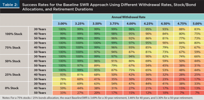
Given a withdrawal rate and retirement duration, we can also look at its success rate, which is the fraction of retirement dates for which PortfolioSim does not exhaust the portfolio value prematurely. Table 2 summarizes the success rate for a variety of withdrawal rates, stock/bond allocations, and retirement durations. Since the SWR calculations are based on historical data, but the future may bring worse conditions (lower returns, higher inflation, correlated stock/bond movement, etc.), the analysis here only considers withdrawal rates to be safe if they have a 100 percent historical success rate.

 

 

 

 

The DMSWR

A detailed understanding of the DMSWR requires a few more definitions. Define a function, IncomeAfterInflation(P, wr, rd, fd), that calculates inflation-adjusted income with a starting income set as a fraction of the initial portfolio value, P. Similar to PortfolioSim, this function is based on an initial withdrawal rate, wr, a retirement date, rd, and a final withdrawal date, fd. It applies observed inflation as calculated from the Consumer Price Index (CPI), or a similar measure, from the retirement date to the final date. The Annual Income (nominal) column in Table 1 shows IncomeAfterInflation(3.57 percent, January 1970, fd) for different final dates. For example, IncomeAfterInflation(3.57 percent, January 1970, January 1980) is $73,478, which is 105.8 percent higher than the initial income due to high inflation during the 1970s.

Current withdrawal rates from the drawdown path can then be computed from the initial withdrawal rate, wr, and the current portfolio value, which depends on the initial portfolio value, P:

Example values for CurrentWR (3.57 percent, January 1970, fd) are shown in the Income Percent column in Table 1. Note that the initial portfolio value, P, is needed to calculate IncomeAfterInflation, but it cancels out when calculating CurrentWR, meaning that any positive value will give the same result.

For a particular retirement date, rd, and final withdrawal date, fd, the DMSWR is the highest withdrawal rate for any safe drawdown path that starts on or before rd and ends with the same fd:

where vd is the “virtual retirement date” of a hypothetical retiree, and (fd – vd) is the length of the hypothetical retirement. Note that to simplify the notation when the retirement date is implied, DMSWR(duration) can be used as shorthand for DMSWR(rd, rd + duration). Regarding the virtual retirement date, there is no theoretical constraint on how far back vd can go, but in practice, it is constrained by the availability of historical data. Due to this practical concern, all results reported in this work are based on a limited lookback period of 20 years.

A key observation is that the DMSWR  succeeds when baseline SWR succeeds since it simply follows the drawdown path using the baseline SWR of a longer retirement duration. Any doubt about the DMSWR directly translates into doubt about the baseline SWR and, consequently, Bengen’s work. Specifically, a retiree using the DMSWR to get a higher withdrawal rate by following the path of a virtual retirement that started on some past virtual retirement date is exactly as safe as a real retiree who actually retired on that date.

Re-Retiring

In the same way that a client can retire by following the safe drawdown path of an earlier retiree, a client can also switch to the safe drawdown path of a new retiree. In other words, if, during retirement, the current DMSWR would provide a higher income than the inflation-adjusted income currently being drawn, a retiree is free to “re-retire” to increase their income. Because the higher withdrawal rate is based on BaselineSWR, it is known to be safe and, thus, the higher income is also safe. Re-retirement is essentially the same idea as the pay out period reset (POPR) technique described by Greaney (2000), except here it is applied to a retiree using the DMSWR instead of the baseline SWR.

Calculating the DMSWR and corresponding income for re-retirement follows much the same process as for initial retirement. Using the current date as the retirement date and the same final withdrawal date, fd, as before, a financial planner calculates DMSWR(today, fd). The annualized income is simply this DMSWR multiplied by the client’s current portfolio value. Since the DMSWR approaches 100 percent as the retirement duration shrinks to zero³, the annual withdrawal rate used for calculating re-retirement income should be capped at a reasonable value (for example, all results in this paper are based on a 20 percent maximum re-retirement withdrawal rate).

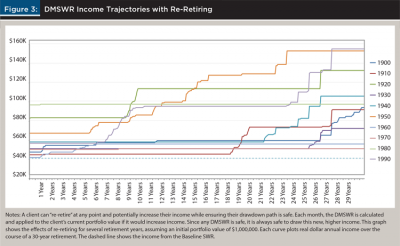
Figure 3 shows the income trajectory over a 30-year retirement for a selection of retirement dates, assuming clients re-retire whenever it’s advantageous. Incomes will never decrease in real terms. In nearly every case, incomes will either start much higher than the baseline SWR, increase during retirement, or both. The benefit of re-retiring depends on the retirement date. For example, there is little benefit for retirements starting in 1930, 1960, and 1970, but there are quite dramatic benefits for retirements starting in 1920, 1950, and 1990.

 

 

 

 

Practical Application and Bond Fund Pricing

DMSWR and PortfolioSim are calculated using the returns of an underlying portfolio. The portfolios modeled here are a blend of an S&P 500 total return index for stocks and constant maturity 10-year treasuries for bonds. The underlying data, along with the Consumer Price Index (CPI) for inflation, are taken from a dataset provided by economist Robert Shiller (2020) that includes monthly data going back to 1871. In the simulations, the portfolio is rebalanced monthly meaning that assets are purchased and sold as needed to maintain the target asset allocation percentages.

Shiller’s dataset includes historical bond data in the form of monthly yield to maturity (YTM) values, which encapsulate the present value of all future coupon payments. For safe withdrawal rate simulations, this YTM data must be converted into monthly bond fund growth rates.

The price of a bond, P_t , at the beginning of month t is calculated as:

where M is the face value, YTM is the yield to maturity, and d_t is the number of years remaining until maturity. To calculate monthly returns, R_t for a bond fund from the YTM data, the price at the end of the month is divided by the price at the beginning of the month. Since the YTM data is for constant maturity 10-year treasuries, d_t = 10 and d_t+1 = 9, which leads to this formula for monthly returns:

This formula implicitly assumes that the YTM of a 10-year bond doesn’t change as the bond ages a month, i.e. that the yield curve is flat. While the yield curve is typically not perfectly flat in practice, this approximation is necessary due to limitations in the available data, and it is commonly accepted by professional practitioners (Morningstar 2008).

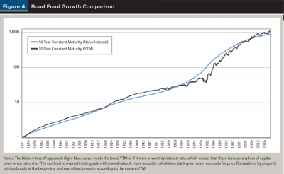
A portfolio of 75 percent stocks and 25 percent bonds produces a baseline SWR (30 years) of 3.69 percent, which is substantially less than the 4 percent rate calculated by Bengen (1994) or the 4.4 percent rate calculated by Kitces (2008). If one assumes that the bonds yield the YTM only as interest, and that the bonds can always be bought and sold at face value, then the resulting baseline SWR (30 years) is much closer to these other works. Historically, however, the fair market value of a 10-year treasury fluctuates substantially, which implies that this assumption is not accurate.

In particular, assuming that the YTM is only paid as interest ignores capital appreciation and depreciation, meaning that a bond fund simulated this way will never lose value unless interest rates are negative (see Figure 4 below). This, in turn, leads to unrealistically high SWR values since the simulated bond fund appears much safer than a real fund. In contrast, the above formula for R_t accounts for bond price fluctuations caused by interest rate changes and leads to more accurate SWR values. Financial planners are encouraged to consider this discrepancy when applying the baseline SWR or DMSWR.

 

 

 

 

While it is relatively straightforward to enter the DMSWR formulas into a spreadsheet, the software used for this work, as well as a large table of past CBSWR, BaselineSWR, and DMSWR values, are provided online by the authors.⁴

Analysis

Unlike the baseline SWR, the DMSWR changes with the retirement date. For a portfolio with an asset allocation of 75 percent stocks and 25 percent bonds, Figure 2 shows the DMSWR for past retirement dates, sampled monthly, for a 30-year retirement. Also shown is the CBSWR, the highest safe withdrawal rate a retiree could have used if they knew the future market returns and inflation. The CBSWR acts as an upper bound on any SWR policy that follows the same withdrawal mechanics. The DMSWR is close to the CBSWR, or at least much closer than baseline SWR, for most of history.

In Figure 2, the DMSWR exceeds the baseline SWR for 90.8 percent of the retirement dates and is equal for all the others. It exceeds the baseline SWR by more than 100 basis points (it’s greater than a 4.69 percent withdrawal rate) for 55.2 percent of historical retirement dates. The average DMSWR is 5.48 percent. And the highest DMSWR was in July 1982 at 13.3 percent.

Keeping in mind the initial goal of addressing Kitces’ starting point paradox, Figure 5 shows a substantial improvement in the stability of initial retirement incomes using DMSWR compared to baseline SWR. The income from baseline SWR follows the market swings. If the portfolio value drops abruptly, then a new retiree’s initial retirement income also drops abruptly.

 

 

 

 

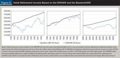
The initial retirement incomes for DMSWR are much smoother and often much higher. There are no cliffs when the stock market drops, only very slight reductions in starting income as the retiree uses a later final withdrawal rate (in the DMSWR formula, fd – vd is slightly longer)⁵. Moderate drops are possible if the best virtual retirement date falls just outside the lookback window (e.g., with a window of 20 years, a drop would appear in February 1986 since the DMSWR calculation can no longer follow the drawdown path of a January 1966 retiree). In practice, financial planners can extend the lookback window to avoid such cases.

Mathematically, the DMSWR is inversely correlated with portfolio value because CurrentWR includes PortfolioSim in the denominator. Thus, when the simulated portfolio value decreases, CurrentWR increases, which will generally lead to higher DMSWR values. This counterbalancing effect causes initial retirement incomes based on DMSWR to be relatively smooth over time.

Following the DMSWR, planners can emphasize to their clients that there is no urgency to retire at a market peak and no penalty for not picking a peak at which to retire. With the DMSWR, market peaks have little effect on retirement income.

 

 

 

 

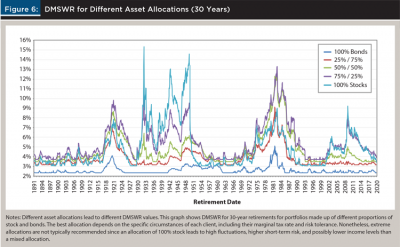
Effects of Asset Allocation

Different asset allocations produce different drawdown paths, different baseline SWR values, and different DMSWR results (see Figure 7 below). The formulas for the DMSWR presume a fixed portfolio asset allocation for simplicity, but there is no such constraint on the technique in general. Instead, financial planners are free to compute the DMSWR for a variety of asset allocations and choose the highest value since all such values are safe. In practice, the decision should be based on the DMSWR, the client’s tax situation, and their current asset allocation.

 

 

 

 

If a client wishes to re-retire then the financial planner is again free to change the asset allocation according to whichever provides the highest withdrawal rate net of fees and taxes. Since the baseline SWR and, thus, the DMSWR, is based on extrapolating from historical data, caution must be taken to avoid overfitting the historical record. In relation to asset allocations, this means that investments fine-tuned for particular sectors, assets, Fama-French factors, etc., may lead to overly optimistic SWR calculations. For example, historical gold returns can be misleading due to the Nixon Shock in 1971, and the historical benefit of small cap value funds may have disappeared. The DMSWR is safe when the baseline SWR is safe, but it does not protect against excessive overfitting and improper extrapolation.

Is the SWR Actually Safe?

The DMSWR is safe in that it follows the drawdown path of a baseline SWR that is safe. It fails if and only if the corresponding baseline SWR also fails.

However, though the baseline SWR has never failed in the years following Bengen’s publication, neither the baseline SWR from Bengen’s work nor the DMSWR are infallible. Both techniques are based on a relatively small sample of data: 1871–2020 is only 149 years, a short duration from which to draw 50-year retirement windows. While using overlapping monthly samples helps, it certainly isn’t as good as a larger set of independent samples.

Even if more historical data were available to bolster the sample size, the future may not be well-modeled by the past, which would invalidate the baseline SWR as well as the DMSWR. Some data is over a century old, and one might realistically believe the world has changed since then. Similarly, unforeseen catastrophes or social change may produce outcomes not covered by history.

Specific to the current economic reality, some commentators have noted that the persistently low yield of U.S. Treasuries in the recent past may be a new regime that prevents us from extrapolating from history. Low yields could imply low bond returns and, assuming a constant risk premium, low stock returns. A retiree could find their portfolio growing less quickly or depleting more quickly and be concerned for their portfolio’s safety. Finke, Pfau, and Blanchett (2013) explored this concern. They estimated a 4.6 percent annualized real return on stocks and –1.4 percent on bonds in the five years following 2013 which, in a scenario using a 50 percent stocks/50 percent bonds portfolio, resulted in a simulated 57 percent failure rate for 2013 retirees. In fact, that 2013 retiree has seen unusually strong portfolio growth during their first five years of retirement. From this, a financial planner might conclude that the baseline SWR and DMSWR are more robust than expected or that the overall economy in 2013 was not especially unique in history, in spite of its exceptionally low treasury yields.

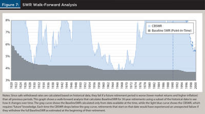
Applying a walk-forward analysis gives us a statistical approach for estimating the failure rate of the baseline SWR by restricting the period of time over which it is calculated.⁷ In other words, for each potential retirement date, the baseline SWR is calculated only using data before that date. The result is then compared to the CBSWR, where a CBSWR lower than the baseline SWR on any particular date indicates a failure.

Historically, the baseline SWR has proven rather robust even on out-of-sample data, as modeled by the walk-forward analysis. For 30-year retirements using a 75 percent stock/25 percent bond allocation, its failure rate is only 2.9 percent since 1920 (see Figure 7). Furthermore, adopting a more conservative approach where retirees use a withdrawal rate 18 basis points lower than the baseline SWR—3.69 percent becomes 3.51 percent —leads to only three failures (0.31 percent), all of which occur for retirements that started in 1929. A reduction of 51 basis points to 3.18 percent produces no walk-forward failures.

There is also longevity risk for the individual. The American Academy of Actuaries (2013) stated that a woman retiring at age 65 and planning a 30-year retirement has a 12 percent chance of outliving her planned retirement. As explored by Finke, Pfau, and Williams (2012), this is somewhat mitigated because most portfolios last longer than the planned 30 years, but to the extent that DMSWR increases incomes and accordingly reduces portfolio values on the final withdrawal date, it exacerbates this problem compared to the baseline SWR method. Re-retiring further reduces portfolio values on the final withdrawal date and so further increases longevity risk. Clients with an opportunity to re-retire may choose to extend their final withdrawal date rather than increase income, and risk-averse clients can plan for a longer retirement and/or apply a downward adjustment to the DMSWR (e.g., reduce their initial withdrawal rate by 25 basis points).

While extending the final withdrawal date or reducing the withdrawal rate can decrease the risk of failure due to out-of-sample longevity or other risk, these solutions are somewhat arbitrary. Methods for monitoring the drawdown path for early detection of potential failures or a more principled understanding of out-of-sample risk would benefit not only the DMSWR but also many of the techniques cited in the literature review.

If the baseline SWR ever fails for some future retirement date and duration, then the DMSWR will also fail for those same retirees. However, the DMSWR extends the risk in that it will also fail for any other retiree following that same drawdown path. So, while it’s true that the DMSWR will fail only if the baseline SWR fails, that failure has the potential to impact many more retirees.

Finally, taxes, investment fees, and other costs are not included in the analysis presented here. Financial planners should include these costs in a client’s expenses and adjust their income accordingly.

Conclusion

The DMSWR offers a substantial improvement over the baseline SWR. Safe withdrawal rates and incomes are often higher and never lower. Real dollar incomes never decrease over time. The DMSWR is safe, as long as the baseline SWR is safe. It addresses the starting point paradox and greatly reduces the need to retire in a peak year to achieve a high income.

The DMSWR does not rely on additional parameters or heuristics that can result in overfitting, nor can it lead to failure in scenarios where the baseline SWR would remain safe. Still, the idea of harmonizing drawdown paths, which is core to addressing the starting point paradox, can be applied to heuristic methods like Klinger’s guardrails (Klinger 2016) or Kitces’ ratcheting rule (Kitces 2015). Exploring the details of such an integration is an opportunity for future work.

The DMSWR is flexible in that it allows “re-retiring” to increase income during retirement, as long as such increases also remain safe.

Overall, the rigorous framework of the DMSWR provides financial planners an opportunity to better serve clients approaching retirement and to continue to serve retirees by monitoring the option to “re-retire” to safely boost their retirement income. 

Endnotes

1. Besides the 4 percent rule, baseline SWR was called SAFEMAX by Bill Bengen in his Financial Advisor Magazine article, “How Much Is Enough,” though this work considers it to be a lower bound and not a maximum. It’s also called the “constant dollar” and “constant inflation-adjusted spending” method, but these descriptions don’t distinguish Bengen’s work from the DMSWR described here.
2. PortfolioSim steps through every month for increased accuracy, but withdrawal rates and incomes are reported using annualized values for convenience.
3. In the extreme case, if a client only plans for a one-month retirement, they can clearly withdraw 100 percent of their portfolio at the beginning of the month since there are no future withdrawals that might fail. 
4. The software implementation is at github.com/minnend/dmswr. Tables of pre-computed CBSWR, BaselineSWR and DMSWR results as well as source data are at bit.ly/2Pf9cR8.
5. In our simulations, very small drops in initial income values occur every 12 months after a useful virtual retirement date. This artifact occurs because BaselineSWR is only calculated for retirement durations that are multiples of one year (12 months). Thus, if a client targeting a retirement of N years follows the drawdown path of a virtual retiree who retired 13 months earlier, the DMSWR is based on BaselineSWR(N + 2 years), not BaselineSWR(N + 13 months). A more fine-grain calculation of BaselineSWR would avoid the initial income dips.
6. For 30-year retirements, CBSWR can only be calculated up to March 1990 (as of March 2020). In Figure 8, CBSWR values after March 1990 represent an upper-bound calculated from the available data.
7. In a walk-forward analysis, a strategy is tested by first running on the earliest data (Jan 1871 – Dec 1919 in this work) and then testing on the next, unused data point (a retirement that begins in Jan 1920). Then the process is repeated by “walking forward” through the data, for example it’s run again on Jan 1871 – Jan 1920 and tested on Feb 1920, run on Jan 1871 – Feb 1920 and tested on March 1920, etc. In this way, statistics are gathered that show when the strategy would have failed in the past given the data available at the time.

References

American Academy of Actuaries. 2013. “Risky Business: Living Longer without Income for Life.” A Public Policy Discussion Paper. Available at www.actuary.org/sites/default/files/files/Risky-Business_Discussion-Paper_June_2013.pdf.

Bengen, William. 1994. “Determining Withdrawal Rates Using Historical Data” Journal of Financial Planning 7 (4): 171–180.

Cooley, Philip L., Carl M. Hubbard, and Daniel T. Walz. “Retirement Savings: Choosing a Withdrawal Rate That is Sustainable.” AAII Journal 20 (2): 16–21.

ERN. 2017. “The Ultimate Guide to Safe Withdrawal Rates—Part 20: More Thoughts on Equity Glidepaths.” Available at earlyretirementnow.com/2017/09/20/the-ultimate-guide-to-safe-withdrawal-rates-part-20-more-thoughts-on-equity-glidepaths/.

Finke, Michael, Wade D. Pfau, and David M. Blanchett. 2013. “The 4% Rule is Not Safe in a Low-Yield World.” Journal of Financial Planning 26 (6): 46–55.

Finke, Michael, Wade D. Pfau, and Duncan Williams. 2012. “Spending Flexibility and Safe Withdrawal Rates.” Journal of Financial Planning 25 (3): 44–51.

Greaney, John. 2000. “Safe Withdrawal Rates—The Pay Out Period Reset (POPR) Method.” Available at retireearlyhomepage.com/popr.html.

Guyton, Jonathan T., and William J. Klinger. 2006. “Decision Rules and Maximum Initial Withdrawal Rates.” Journal of Financial Planning 19 (3): 50–58

Kitces, Michael E. 2008. “Resolving the Paradox—Is the Safe Withdrawal Rate Sometimes Too Safe?” The Kitces Report. Available at www.kitces.com/may-2008-issue-of-the-kitces-report/.

Kitces, Michael E.  2015. “The Ratcheting Safe Withdrawal Rate—A More Dominant Version of the 4% Rule?” Nerd’s Eye View. Available at www. kitces.com/blog/the-ratcheting-safe-withdrawal-rate-a-more-dominant-version-of-the-4-rule/.

Klinger, William J. 2016. “Guardrails to Prevent Potential Retirement Portfolio Failure.” Journal of Financial Planning 29 (10): 46–53.

Morningstar. 2008. “Return Calculation of U.S. Treasury Constant Maturity Indices.” Morningstar Methodology Paper. Available at admainnew.morningstar.com/directhelp/Morningstar_UST_Constant_Maturity_Return_Methodology.pdf.

Pfau, Wade D. 2013. “A Broader Framework for Determining an Efficient Frontier for Retirement Income.” Journal of Financial Planning 26 (2): 44–51.

Pfau, Wade D. 2016. “Does the 4% Rule Work Around the World?” Forbes Available at www.forbes.com/sites/wadepfau/2016/06/29/does-the-4-rule-work-around-the-world/#6ef460555e29.

Pfau, Wade D. Sept. 2017. How Much Can I Spend in Retirement?: A Guide to Investment-Based Retirement Income Strategies. McLean, Va.: Retirement Researcher Media.

Shiller, Robert 2020. Online Data Robert Shiller. The “U.S. Stock Markets 1871-Present and CAPE Ratio” Dataset. Available at www.econ.yale.edu/~shiller/data.htm.

Zolt, David 2013. “Achieving a Higher Safe Withdrawal Rate with the Target Percentage Adjustment.” Journal of Financial Planning 26 (1): 51–59.

Citation

Marwood, David, and David Minnen. 2020. “Safely Boosting Retirement Income by Harmonizing Drawdown Paths.” Journal of Financial Planning 33 (11): 46-60.