How Do Commodities Fit into Client Portfolios?

Journal of Financial Planning: October 2022

 

Executive Summary

• Academic literature suggests that since the mid-2000s, improved investment technology may have resulted in the “financialization” of commodity markets. This financialization is defined as the participation in commodity markets of institutional investors that have not historically been part of the commodity trading complex. Whether due to financialization or not, since 2005, the correlation structure of commodities with other assets, and perhaps their expected returns, has been altered. This paper summarizes these changes, and their implications for investment planning.
• Since 2005, return correlation between the Bloomberg Commodities Index and the S&P 500 has been 49 percent, compared to –30 percent 1973–2004. This change has significantly reduced the ability of commodities to contribute to an efficient portfolio in a modern portfolio theory framework.
• The correlation of returns to the Bloomberg Commodities Index with inflation has been very high since 2005, at 64 percent. This correlation comes primarily from the correlation of commodities with unexpected inflation. The index is slightly negatively correlated with inflation expectations. This is in contrast to pre-2004, when commodities returns were correlated with both expected and unexpected inflation. Commodities’ high correlation with unexpected inflation makes the asset class an appealing inflation hedge despite its limited contributions to an efficient portfolio.

Jason D. Fink, Ph.D., is the Wachovia Securities faculty fellow and a professor in the department of finance and business law at James Madison University College of Business. He is also director of research with Graves Light Lenhart Private Wealth Management in Harrisonburg, Virginia.

Kristin E. Fink, Ph.D., is a College of Business foundation fellow and a professor in the department of finance and business law at the James Madison University College of Business.

The authors thank Asa Graves and Ash Heatwole for valuable discussions that led to significant improvements in this work. We are also thankful for the contributions of an anonymous reviewer who provided key insights. This work was supported by the College of Business, James Madison University.

JOIN THE DISCUSSION: Discuss this article with fellow FPA Members through FPA's Knowledge Circles​. ​​​

FEEDBACK: If you have any questions or comments on this article, please contact the editor HERE. 

NOTE: Click on the images below for PDF versions

The standard stock–bond portfolio mix remains the bread-and-butter combination of investment vehicles for the financial planning community, even as the search for assets to complement these fundamental building blocks of client portfolios continues. Over the past 20 years, the investment infrastructure around commodities has transformed the asset class in such a way as to substantially improve the feasibility of client participation. Further, recent insights regarding the long-term behavior of gold prices can be extended to the broader class of commodities, providing a basis for the formation of return expectations for the asset class. However, coincident with the decreased cost of commodity exposure and increased access for clients, there has also been a change in the fundamental investment profile of commodities. These changes include increased correlation with equities, which are typically the primary driver of client returns and risk, as well as a change in the components of inflation with which commodities exhibit correlation. This paper reviews these developments and synthesizes the implications for financial planners attempting to use the commodity asset class to improve client portfolios. This synthesis is particularly important given the recent attention paid to commodities as a result of the elevated inflation environment.

Gorton and Rouwenhourst (2006, hereafter GR) found that commodities possess several characteristics desirable for investors; most notably that prior to 2004, commodities as a class had a favorable correlation structure with both stocks and bonds, as well as a desirable Sharpe ratio. For example, they find that while the Sharpe ratio for a basket of commodities exceeded both the S&P 500 and a collection of bonds over their period of study, the basket of commodities had a correlation of –0.06 and –0.27 with stocks and bonds respectively.¹ However, even the simple commodity trading strategy of GR is costly to implement. Among other drawbacks, the strategy is labor-intensive and necessitates investors manage the “roll” of futures contracts. Since 2006, ETFs have been introduced that undertake these kinds of commodity transactions on behalf of the fund holders at a reasonable cost. While commodity ETFs have higher fees than correspondingly well-managed equity funds, the value-weighted average expense ratio for commodity ETFs are roughly 0.69 percent.² Plante and Roberge (2007) was an example of early work exploring the benefits of the then-newly introduced commodity ETFs.

Do the Return Patterns of Commodities Still Hold Post-Financialization?

With such easy exposure to commodity strategies via low-cost ETFs, an important consideration is whether the benefits of adding commodities to a portfolio outlined in Gorton and Rouwenhourst (2006) continue to hold. As discussed in Büyükşahin and Robe (2014), the entrance of (typically passive) institutional investors who weren’t traditionally part of the commodity ecosystem into commodity markets is referred to as the “financialization” of the commodity markets. While academic debate about the impact of financialization on changes to the joint distribution of commodities returns continues, Büyükşahin and Robe (2014) specifically find that trader motivation does indeed affect the return distribution of commodities and equities. Basak and Pavolova (2016) further provide a theoretical model that suggested that correlations between commodity indices and equity indices should increase as a result of such financialization, reducing the benefit of diversification into commodity markets by those with traditional stock–bond portfolios.

In this paper, several variables of interest are collected at a quarterly frequency from June 1973–June 2022. This is a period with over 35 years pre-financialization and more than a decade and a half post-financialization of commodities. Comparability of the findings here to GR is important. However, GR begin their analysis in 1959. With the elimination of the gold standard in 1973, the relationship between a basket of commodities and the dollar fundamentally changed—especially, but not only, since broad baskets of commodities include substantial amounts of gold. Since the gold standard is highly unlikely to return, it is prudent to begin the analysis here sometime after its elimination.³ To maximize the data set since this shift in financial regime, this analysis begins in Q1 1973, the first quarter in which the value of gold was allowed to freely float in the United States. The data concludes in Q2 2022.

From Bloomberg, quarterly returns to the S&P 500 Total Return Index (SP500), the Bloomberg Commodity Total Return Index (BCOM), and the Bloomberg Aggregate Bond Index (BBOND) are collected, which are used as proxies for returns to equities, commodities, and bonds, respectively.⁴ From Bloomberg, inflation data is gathered in the form of the U.S. CPI for all urban consumers (CPI), and the percentage change in CPI each quarter (CPI_D%) is computed.⁵ We collect our historical data for the risk free rate from Q1 1973–Q4 2020 from the Fama–French Factors and Portfolios dataset via Wharton Research Data Services (WRDS). Since that data is available monthly and constructed from U.S. Treasury one-month bills, and the data frequency for our dataset is quarterly, the series is aggregated to form a quarterly risk-free return. To extend this data into 2022, the risk-free rate series for that year is augmented with the three-month constant maturity U.S. Treasury data from the St. Louis Fed.⁶ The risk-free rate is denoted RISK_FREE. Finally, the real price of BCOM (Real_BCOM) is constructed and defined by BCOM/CPI.

In Table 1, we see descriptive statistics for the variables for three periods: 1973–2004 (roughly the GR period of study, and seen in Panel A), 2005–2022 (seen in Panel B, the time since the GR study and in line with the post-financialization of commodities), and the entire period, 1973–2022 (seen in Panel C). Several results are worth noting. The positive performance of commodities presented in GR are tempered throughout, and particularly so since 2005. Though muted, the 1973–2004 results are qualitatively similar to Gorton and Rouwenhourst (2006). For example, GR found Sharpe ratios of 0.38, 0.26, and 0.43 for stocks, bonds, and commodities, while in Panel A Sharpe ratios of 0.176, 0.162, and 0.196 are seen. The biggest difference between the findings presented here and those of GR is in the lower risk-adjusted returns to the assets, particularly stocks and commodities.

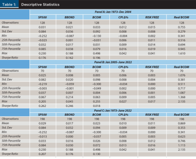
Panel B illustrates the results since the GR study, and it is seen that the performance of a basket of commodities was much lower in this period. The Sharpe ratios of stocks and bonds over this 17-year period were 0.262 and 0.246, respectively. Both of these are notably higher than in the earlier period. Commodities, by contrast, had a Sharpe ratio of 0.018, indicating that the BCOM rate of return was just in excess of the risk-free rate. Not reported in the table is that this underperformance was to some extent driven by a pair of devastating back-to-back quarters in the second half of 2008, when BCOM lost about 30 percent of its value in Q3 and Q4 2008. However, even excluding these two quarters (which of course, an investor would have been quite lucky to do), the Sharpe ratio would still be less than half of the other two asset classes.

Panel C provides the descriptive statistics for the overall four-and-a-half-decade period of this analysis. The mean quarterly return for the S&P 500 is 2.9 percent, which is higher than commodities and bonds. Bonds and commodities have somewhat similar mean returns, at 1.7 percent and 2.3 percent respectively. However, the return premium that commodities exhibit over bonds comes at a substantial volatility cost. Commodities’ return standard deviation over the entire period is 0.094 (which exceeds even equities), compared to 0.032 for bonds. Therefore, despite the strong outperformance in Panel A, commodities’ Sharpe ratio lags in the overall period due to the substantial return underperformance of the last 18 years coupled with elevated standard deviation throughout. Over the entire period, the Sharpe ratios of stocks, bonds, and commodities respectively are about 0.207, 0.176, and 0.130. Over the last 55 years, commodities have not been a particularly attractive standalone investment.

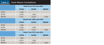
However, even a relatively inefficient (low Sharpe ratio) asset can be of value to an investor, so long as it is imperfectly correlated with the returns of other assets. GR found (with their quarterly data from 1959–2004) that commodities have a correlation with stocks of –0.06 and –0.27 with bonds, making commodities a particularly attractive diversifier in the context of most retirement portfolios.

Table 2 presents correlations between stocks, bonds, and commodities for the same periods presented in Table 1. Panel A finds (unsurprisingly) that the correlation structure in the 1973–2004 period exhibits patterns similar to the GR results. Specifically, commodities exhibited correlations with stocks and bonds of –0.30 and –0.22, respectively. Unfortunately, this structure appears to have changed rather dramatically in the last 18 years, as seen in Panel B. Since 2005, the correlation of commodity returns with stocks has spiked to 0.49, though the negative correlation of commodities to bonds has held up, and even usefully fallen a bit, to –0.27. Panel C provides the correlation structure for the entire 1973–2022 period. The contrast of Panels A, B, and C illustrate the degree to which the correlation structures may change and suggest the insufficiency of financial planning that assumes otherwise.

For example, Figure 1 illustrates the dynamic correlation between stocks and commodities over the entire period using a backward-looking, rolling four-year window for the estimation. During the pre-2005 period, it is clear that SP500–BCOM correlation is low, consistent with Panel A of Table 2. But even in this period, there are notable stretches in which the correlation is elevated—most notably in the early 1980s.

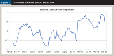
Beginning at the time of the great financial crisis, the correlation between BCOM and SP500 elevated, and remained elevated through 2022 (on a rolling four-year basis). What is the driver behind this remarkable shift in structure? Several papers find that commodity market financialization is behind this trend. For example, Adams, Collot, and Kartsakli (2020) find empirically that financial variables are the primary drivers behind commodity market return and volatilities since 2004. This is directly in line with the theoretical model of Basak and Pavolova (2016), who further find that the correlation between equity and commodity markets should increase along with financialization. Interestingly, Adams, Collot, and Kartsakli (2020) find a modest decline in the degree of financialization in the late teens, and this corresponds to a slightly lower correlation between BCOM and SP500 over that period. These findings, if confirmed, are disappointing news to financial planners. They imply that the very instruments designed to facilitate broader investment in commodities are the culprits reducing the diversification benefit of the asset class.

Of course, the time frame of 2004–2022, while almost two decades, is relatively short in the context of long-run asset class joint distributions, and there remains academic debate as to whether financialization is indeed the driver of the changes. For example, Bhardwaj, Gorton, and Rouwenhourst (2016) argue that the evidence in favor of financialization being the primary driver may also be explained as simply a business cycle effect, while Chari and Christiano (2017) find that net financial flows do not sufficiently explain the characteristics of commodity returns. Identifying the source of the changes in the statistical behavior of commodity returns is an important academic topic since proper identification will allow better understanding of when the distributions may change again. Putnam (2018) provides an excellent review of the state of this discussion in the academic literature. Most important to current financial planners, however, is that substantial changes have taken place that cause the distribution of commodity returns to be quite different over the past 20 years when compared to the GR study period.

What Are the Implications of the Shift in the Return and Correlation Structure of Commodities?

Higher correlation and lower returns naturally imply that commodities have been a substantially less effective diversifier since 2005 than studies employing earlier data would suggest. Figure 2, Panel A illustrates the efficient frontier that was possible through an allocation of SP500, BBOND, and BCOM in the period 1973–2004.⁷ In addition to the efficient frontier, five other portfolios are referenced. As a benchmark, a “typical” 60–40 stock–bond portfolio is denoted 60–40–0, using the nomenclature to be used to identify a portfolio with SP500/BBOND/BCOM percent holdings in each asset class. The all-stock, all-bond, and all-commodity portfolios are also labeled. It is worth noting that the 60–40–0 portfolio is well inside the efficient frontier, and so we also compute the efficient portfolio with the same standard deviation as the 60–40–0 portfolio. It turns out that the resulting efficient portfolio consists of 37 percent invested in SP500, 0 percent invested in BBOND, and 63 percent invested in BCOM. Therefore, the final labeled portfolio in Panel A is the 37–0–63 portfolio.⁸ In this early period, the 37–0–63 portfolio is not an unusual one to be found along the efficient frontier for relatively high volatility portfolios. Though 63 percent of the portfolio would no doubt be considered too distant from the “standard” portfolio approach for most financial planners, this allocation is a natural consequence of the Sharpe ratios seen in Table 1 along with the correlation structure.

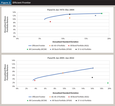
As would be expected from the Sharpe ratios and correlation structure presented in Tables 1 and 2, the efficient frontier in the 2005–2022 period presented in Panel B of Figure 2 looks quite different from the one in Panel A. A first glance clearly indicates that the entire frontier shifts lower. What isn’t necessarily evident at first glance is that commodities have all but disappeared from the efficient frontier. It is instructive to notice that the 60–40–0 portfolio now resides firmly on the efficient frontier, and to contrast that with the location of the 37–0–63 portfolio that is now well on the interior of the set, indicating significant inefficiency. This formerly efficient portfolio now provides a lower return for much greater risk than the 60–40–0 benchmark. This makes intuitive sense, as the all-commodity portfolio in Panel B can now be seen in the lower right corner. Only the very lowest risk-efficient portfolios incorporate any commodity exposure—those with standard deviations less than about 4 percent, and the BCOM allocation is rarely above low single-digit percentage allocations in an efficient portfolio.

Both the correlation structure and the realized returns contributed to the decline in the diversification benefit of commodities. The academic debate continues concerning the reasons for the change in the correlation structure, with financialization perhaps the leading theory.⁹

Interestingly, a different strand of recent literature has suggested a route by which one may be able to form expected returns for commodities over an intermediate horizon. This approach is behavioral in origin, and it suggests a link between expected commodity returns and the real price of commodities.

The Real Price of Commodities and Expected Returns

Many studies have found that the returns to commodities tend to mean-revert in the long run. For example, Andersson (2007) examines hedging errors from a wide variety of individual commodity prices from around the globe to determine that they are mean reverting, while Yang, Goncu, and Pantelous (2018) find return reversals in Chinese commodities markets are commonplace. Zaremba, Bianchi, and Mikutowski (2021) provides a particularly effective long-dated study of U.S. and English commodity prices going back seven centuries that finds strong evidence of mean reversion in individual commodity returns. There is some evidence, however, that this mean reversion is stronger in spot rather than futures markets (Chaves and Viswanathan 2016).

Applying more specific structure to the nature of this mean reversion, Erb and Harvey (2013) and Erb, Harvey, and Viskanta (2020) suggest that gold appears to mean-revert to a stable real price. While gold may be bid up in times of economic uncertainty, and neglected in times of relative prosperity, it tends to revert to a long-run established real price. In this sense, the real price of gold plays a role similar to that of CAPE with equities. If this relationship is stable, it means that there is potentially an ability to forecast returns to gold that are both a gross violation of efficient markets and a basis for forming return expectations to the asset.

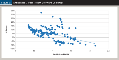
Carpantier (2021) called the stability of this relationship for gold into question, but reaffirmed its stability for a broad cross section of 17 other commodities. This is explored further in Figure 3, which examines the relationship between Real_BCOM (which is composed of many of the commodities studied in Carpantier (2021)) and the expected returns to BCOM. The vertical axis of this scatterplot provides the annualized seven-year-forward realized returns to BCOM (which we will denote BCOM_7RET), while the horizontal axis gives Real_BCOM.¹⁰ The relationship is striking, given that the efficient markets hypothesis would suggest that no relationship should exist at all. The fitted line gives us the estimated relationship between BCOM_7RET and Real_BCOM:   

   (1)        BCOM_7RET = 0.152 – 0.109 * Real_BCOM                     

So long as this relationship is stable, it gives us the conditional expectation of BCOM_7RET, and can be used for the formation of expected returns. For example, if Real_BCOM is 250.855 / 295.328 = 0.849 (which it was at the conclusion of Q2 2022), this implies an expected annual return of 0.152 – 0.109 × 0.849 = 5.94 percent for commodities over the next seven years.

Optimal Portfolios Using Real_BCOM to Form Expected BCOM Returns

If financialization is the driver of the new correlation structure of commodity returns, then BCOM is locked into an environment that works against inclusion of commodities in client portfolios relative to the suggestions of earlier work. However, what is clear from the estimated relationship between BCOM_7RET and Real_BCOM given in Equation (1) is that there are times that BCOM can be a contributing component of an efficient portfolio. Namely, this is true when Real_BCOM is relatively low. The degree to which BCOM will provide an efficient route to add value to client portfolios will, however, depend crucially on its real price and the joint distribution of asset returns. A few examples will illustrate the extent to which BCOM is likely to contribute to an efficient portfolio.

The analysis proceeds here with several assumptions in place. First, assume that the correlation structure of SP500, BBOND, and BCOM, as well as the expected returns to SP500 and BBOND are taken from the unconditional statistical estimates of the period 2005–2022. This implies that the correlation structure is given in Table 2 Panel B, and that the expected returns for SP500 and BBOND are their respective means given in Table 1 Panel B. Certainly, these assumptions could be questioned, and they are only a rough approximation of the modern environment. However, they provide a reasonable framework of a post-financialization commodity market and its interrelationship with equity and bond markets for the purposes of the examples. Second, assume that expected returns to BCOM are governed by the relationship between expected returns and Real_BCOM given in Equation (1).

Table 3 provides comparisons of efficient portfolios formed with and without the inclusion of commodities in the portfolio under these assumptions, for several different historical values of Real_BCOM. As a set of comparison portfolios, four “standard” portfolios with different degrees of risk are constructed. These portfolios are formed from only SP500 and BBOND. These portfolios are arbitrarily labeled Ultraconservative (a 10 percent stock, 90 percent bond portfolio), Conservative (30–70), Balanced (50–50), and Aggressive (70–30). The annualized portfolio standard deviations and expected returns for these portfolios are provided in Panel A. Since BCOM is not used in the formation of these portfolios, the value of Real_BCOM does not affect the standard deviations or expected returns of these portfolios.

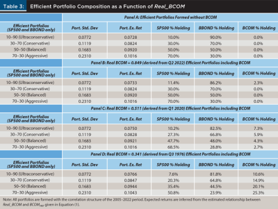
In Panels B, C, and D, the portfolios in Panel A are augmented by allowing investment in BCOM. Efficient portfolios are selected by matching the standard deviations of each of the four portfolios from Panel A while maximizing expected returns of the portfolio. In this way, the four base portfolios can be viewed as “constrained” choices, where the constraint is that BCOM exposure must be zero. This allows examination of the effect on the efficient portfolios when that constraint is relaxed. Of course, to undertake the determination of the efficient portfolios, one must know the expected return to BCOM, which is contingent on Real_BCOM.

In Panel B, Real_BCOM is set equal to 0.849, which was the value of Real_BCOM at the conclusion of Q2 2022. This is a slightly below “typical” value for Real_BCOM, as its mean value from 2005–2022 was about 1.07. From Equation (1), this implies an annualized expected return of about 5.94 percent. The resulting expected portfolio returns may be seen in the second column, while the corresponding optimal holdings of SP500, BOND, and BCOM may be seen in the third, fourth, and fifth columns. The potential inclusion of commodities in the portfolio has negligible effect on the efficient portfolios chosen. It is only for the lowest risk portfolio that commodities are included at all, and even then, only 2.3 percent of the portfolio is so allocated, resulting in an increased expected return for the Ultraconservative portfolio of only five basis points. Since any value for Real_BCOM greater than 0.849 will result in an even lower expected return, it appears that inclusion of commodities in the portfolio is unlikely to be efficient for most portfolios, most of the time.

In Panel C, the hypothetical value for Real_BCOM is set to a recent nadir, at the conclusion of Q1 2020. At this moment in time Real_BCOM was 0.511, about a standard deviation below its 1973–2022 mean. Applying Equation (1), this implies an annualized expected return of about 9.29 percent, almost double the expected return from Q2 2022. Despite this substantially greater expected return, we can see in the table that the optimal commodity holdings for the various efficient portfolios in Panel C are still quite low. In all cases, the efficient ex ante holdings are between 2 percent and 8 percent. Since the holdings are so low, portfolio expected returns are once again negligibly affected. At first glance, this result from a portfolio optimization may seem surprising. However, note that even in this heightened expected return environment for commodities, the ex ante expected annualized nominal return for BCOM is 9.29 percent, which is less than the SP500 ex ante expected annualized nominal return of 12.11 percent. Further, BCOM has a greater standard deviation than SP500 (0.098 versus 0.082) and a correlation with SP500 of about 0.49. More sophisticated analysis may lead to allocations that include commodities to a greater extent. For example, SP500 forecasts in high-equity-valuation markets may provide lower return expectations than our example here. Nonetheless, the correlation structure post-2005 appears to have given rise to a quite difficult environment for those hoping to diversify with commodities.¹¹

For a look at the environment most likely to heavily favor commodities, next consider a Real_BCOM value of 0.341, which is the lowest value observed in our data set, seen in Q3 1976 (continue to assume the post-financialization correlation structure in this example). This level of Real_BCOM implies an expected return of 11.48 percent, and results in the efficient portfolio allocations seen in Panel D. In this most extreme favorable-to-commodities environment, substantive allocations are indeed made to BCOM. The more aggressive the portfolio, the greater the allocation to commodities in this environment. Further, the allocations toward BCOM come primarily by reducing the allocation toward equities, having the effect of tempering the portfolio standard deviation due to the imperfect correlation between SP500 and BCOM. And yet, despite this increased allocation, even in this commodity-favorable environment, the expected return increases to the portfolios remain muted. The Aggressive portfolio allocates 25.3 percent of the portfolio to commodities, and in doing so increases portfolio expected returns by an annualized 0.27 percent. The other three portfolios exhibit even less improvement in their expected returns.

Again, the specific assumptions made in these examples are just that—assumptions. However, what appears to be a significant driver of the decreased effectiveness of commodities as a useful source of portfolio diversification is the heightened correlation of commodities with equities since 2005. According to Basak and Pavolova (2016), this is an effect that would be expected from the financialization of commodities markets. If financialization is indeed the source of this heightened correlation, it is expected that markets will continue this behavior that is so evident in Figure 1 in the post-GR period. So long as that elevated correlation continues, one would expect relatively muted benefits from the inclusion of commodities in equity-heavy portfolios.

Correlation with Inflation

One of the common uses of commodity investments, and one that does not show up explicitly in portfolio optimizations using nominal returns, is to provide a partial inflation hedge. Naturally, this can be an important consideration with client portfolios, particularly for those clients already in the retirement stage. GR document that commodity returns are positively correlated with inflation. Further, they find that when inflation is decomposed into expected and unexpected components, commodity returns are positively correlated with each of these as well. This correlation is relatively weak, but statistically significant. In the GR study this is in contrast with other asset classes. They found the returns to both stocks and bonds negatively but weakly correlated with inflation.

GR used the three-month Treasury bill rate in a given quarter as the expected inflation rate for the subsequent quarter, and then used this to decompose realized inflation into expected and unexpected inflation. With the advent of quantitative easing, the rationale for the three-month T-bill rate as a proxy for inflation has become weaker. A better (but like any source, still imperfect) measure of expected inflation is the lagged value of expected inflation from the University of Michigan.¹²  This survey is published monthly and is available back to 1978. For this analysis, the final value each quarter is taken as the forward-looking expectation of (annualized) inflation next quarter. Denote this series MICH. From 1978–2022, this series has a correlation of 0.80 with realized quarterly changes in CPI. By comparison, lagged three-month Treasury bill rates have a 0.53 correlation with realized quarterly changes in CPI. For this reason, this analysis uses MICH to decompose inflation into expected and unexpected components. Denoting unexpected inflation as UNEXPECTED, it can be recovered using the following formula:

   (2)           UNEXPECTED_t = CPI_t  – MICH_t-1

Since CPI and MICH are observed, the UNEXPECTED series may be constructed directly. The distinction between expected and unexpected inflation is subtle but important. By using MICH to form forecasts of next-quarter CPI, we are proxying for the market expectation of inflation. As asset prices are forward looking, we anticipate that expected inflation is already embedded in their values. Unexpected inflation, by contrast, may well be a driver of inflation-sensitive asset returns. By forming UNEXPECTED as the residual of CPI and MICH in Equation (2), we are able to capture this unanticipated component.

Table 4 illustrates the relationships between CPI, MICH, and UNEXPECTED with asset returns. Since this analysis uses the lagged value of MICH in Equation (2), the lagged value of MICH is presented in Table 4. In the pre-financialization period of 1973–2004, BCOM does provide an interesting inflation-hedge profile. The asset class does exhibit a contemporaneous correlation with CPI of 0.287, and the correlation is similar with unexpected CPI. This is a potential argument in favor of keeping some commodity holdings in a portfolio at all times—commodity returns are only correlated with expected inflation (MICH) at a low level of 0.104, but when unexpected inflation strikes, commodities provide a higher degree of correlation that can help out the portfolio. The argument is buttressed by the low and mostly negative correlations between stock and bond returns and the inflation variables. There is, however, an important caveat. These correlations are relatively short term. BCOM_7RET is negatively correlated with all three inflation variables, providing some indication that the returns to commodities may mean-revert following inflation spikes.

This argument for keeping some commodities in the portfolio for unexpected inflation shocks may be even stronger post-financialization. From 2005–2022, the correlation between BCOM and CPI is notably higher, at 0.640. Even more pronounced is the decline in the correlation of BCOM with expected inflation proxied by MICH (–0.156) and the increase in the correlation between BCOM and unexpected inflation (0.690). To the extent positive inflation is a surprise, BCOM has a strong tendency in the direction of positive returns. Interestingly, SP500 also exhibits a similar pattern, though less correlated with UNEXPECTED. Commodities post-financialization have been the better hedge against unexpected inflation, but stocks have also been rather effective in this regard. Indeed, in 2005–2022, stocks hedged unexpected inflation similarly to how commodities did from 1973–2004. Unsurprisingly, bonds were generally not a desirable place to be in an inflationary environment. Finally, BCOM_7RET continues to be negatively related to inflation variables post-financialization, indicating that the temporary nature of the commodity returns with inflation appear to have remained.

Conclusion

The correlation structure of the asset classes of equities, bonds, and commodities appears to be quite different post-2005 compared to the pre-2005 period described by Gorton and Rouwenhourst (2006). The post-2005 period has exhibited lower commodity returns and substantially higher commodity–equity return correlations. Both of these shifts directly affect the degree to which commodities are useful diversifiers for the benchmark efficient portfolios often recommended by financial planners. While commodities may still provide a useful contributor to diversification, their benefit appears to be present in only certain circumstances.

One leading theory for why commodities may have lost some of their diversification appeal lies in their financialization since 2005. Commodities are substantially less complicated and costly for financial advisers to invest in as an asset class on behalf of clients than was the case previously. Several large commodity funds now exist, and it is possible to invest in the asset class with expense ratios less than 50 basis points and without detailed knowledge of the functioning of commodities markets. If financialization is the explanation for these changes, it is ironic. The real cost of these funds may well be that their existence may have shifted the correlation structure of commodities with equities post-financialization, rendering the asset class considerably less attractive than the pre-2005 period.

However, while the increased correlation of commodities with equities disrupts their usefulness for the formation of efficient portfolios in the context of modern portfolio theory, the correlation of commodities with unexpected inflation is elevated in the post-financialization period. Interestingly, commodity returns over the 2005–2022 period are negatively related to inflation expectations. However, with a 69 percent correlation with unexpected inflation they have potential to be quite useful as an inflation hedge. 

Endnotes

1. These values were measured at a quarterly return frequency.
2. Source: Valueline ETF Screener.
3. Precious metals are currently about 20 percent of the Bloomberg Commodity Index. Cashin and McDermott (2002) find that the variances of real commodity prices changed after the demise of the gold standard in the early 1970s. Further, Bordo (1993) finds that the inflation regime is more stable in the post-Bretton Woods era while Cuddington and Liang (1998) find that flexible-exchange regimes are associated with higher real commodity price volatility. These shifts indicate that econometric inference would be biased if the pre-1973 regime were included in the analysis. For an excellent brief review of the gold standard in the United States, see Elwell (2011).
4. The Bloomberg tickers for the return series are SPXTR Index, BCOMTR Index, and LBUSTRUU Index, respectively. SPXTR Index is not available prior to June 1988. For 1976–1988, we use SPX Index returns for SPXTR Index. For periods in which the two series overlap, their correlation is 0.9999995. In all cases, we use total returns including dividend/coupon payments. BCOMTR is not available prior to June 1976. For quarters prior to this, ICE BofA US Corporate Index Total Return Index (identifier BAMLCC0A0CMTRIV from the St. Louis Federal Reserve) is substituted. The correlation between these two series when they overlap is approximately 93 percent.
5. The Bloomberg ticker for our inflation data is CPI INDX Index.
6. See https://fred.stlouisfed.org/series/DGS3MO.
7. Though still constructed from the quarterly data, please note that for the efficient frontiers in the figures, all values have been annualized, thus the difference in the returns and standard deviations seen in the “all stock” and “all bond” portfolios from the corresponding descriptive statistics in Table 1 Panel A (which are on a quarterly scale).
8. Portfolio weights are rounded to the nearest percent for simplicity.
9. In addition to the Büyükşahin and Robe (2014), Basak and Pavolova (2016), and Adams, Collot, and Kartsakli (2020) papers that we cited earlier in the paper that explore this issue, see for example Silvennoinen and Thorp (2013), Cheng and Xiong (2014), and Singleton (2014).
10. The seven-year forward return (r_C) at a given point in time is computed as the geometric quarterly return for the subsequent 28 quarters (no past or contemporaneous returns are included, this is entirely forward-looking).  This return is then annualized as:                         
11. Interestingly, BCOM substantially outperformed expectations in the year following Q1 2020, returning 34.9 percent. SP500 outperformed to an even greater degree, returning 56.4 percent.
12. See https://fred.stlouisfed.org/series/MICH.

Citation

Fink, Jason D., and Kristin E. Fink. 2022. “How Do Commodities Fit into Client Portfolios?” Journal of Financial Planning 35 (10): 78–93.

References

Adams, Zeno, Solene Collot, and Maria Kartsakli. 2020. “Have Commodities Become a Financial Asset? Evidence From Ten Years of Financialization.” Energy Economics 89: 104769.

Andersson, H. 2007. “Are Commodity Prices Mean Reverting?” Applied Financial Economics 17 (10): 769–783.

Basak, Suleyman, and Anna Pavlova. 2016. “A Model of Financialization of Commodities.” Journal of Finance 71 (4): 1511–1555.

Bhardwaj, Geetesh, Gary B. Gorton, and K. Geert Rouwenhorst. 2016. “Investor Interest and the Returns to Commodity Investing.” Journal of Portfolio Management 42 (3): 44–55.

Bordo, Michael B. 1993. “The Bretton Woods International Monetary System: A Historical Perspective.” In A Retrospective on the Bretton Woods System: Lessons for International Monetary Reform. Edited by Michael B. Bordo and Barry Eichengreen. University of Chicago Press.

Büyükşahin, Bahattin, and Michel A. Robe. 2014. “Speculators, Commodities and Cross-Market Linkages.” Journal of International Money and Finance 42 (1): 38–70.

Carpantier, Jean-Francios. 2021. “Anything but Gold—The Golden Constant Revisited.” Journal of Commodity Markets 24: 100170.

Cashin, Paul, and C. John McDermott. 2002. “The Long-Run Behavior of Commodity Prices: Small Trends and Big Variability.” IMF Staff Papers 49 (2): 175–199.

Chari, V.V., and L. Christiano. 2017. “Financialization in Commodity Markets.” NBER Working Paper No. 23766.

Chaves, Denis, and Vivek Viswanathan. 2016. “Momentum and Mean-Reversion in Commodity Spot and Futures Markets.” Journal of Commodity Markets 3 (1): 39–53.

Cheng, Ing-Haw, and Wei Xiong. 2014. “Financialization of Commodity Markets.” Annual Review of Financial Economics 6 (1): 419–441.

Cuddington, John T., and Hong Liang. 1998. “Commodity Price Volatility Across Exchange Rate Regimes.” Georgetown University Working Paper.

Elwell, Craig K. 2011. “Brief History of the Gold Standard in the United States.” Congressional Research Service, Publication No. R41887.

Erb, Claude B., and Campbell R. Harvey. 2013. “The Golden Dilemma.” Financial Analysts Journal 69 (4): 10–42.

Erb, Claude B., Campbell R. Harvey, and Tadas Viskanta. 2020. “Gold, The Golden Constant, and Déjà Vu.” Financial Analysts Journal 76 (4): 134–142.

Gorton, Gary, and Geert Rouwenhourst. 2006. “Facts and Fantasies About Commodity Futures.” Financial Analysts Journal 62 (2): 47–68.

Plante, Jean-Francios, and Mathieu Roberge. 2007. “The Passive Approach to Commodity Investing.” Journal of Financial Planning 20 (5): 66–75.

Putnam, Kyle. 2018. “Financialization of Commodity Markets.” In Commodities: Markets, Performance, and Strategies. Edited by H. Kent Baker, Greg Filbeck, and Jeffery H. Harris. Oxford Academic: 490–514.

Silvennoinen, Annastiina, and Susan Thorp. 2013. “Financialization, Crisis, and Commodity Correlation Dynamics.” Journal of International Financial Markets, Institutions, and Money 24 (2): 42–65.

Singleton, Kenneth. 2014. “Investor Flows and the 2008 Boom/Bust in Oil Prices.” Management Science 60 (2): 300–318.

Yang, Yurun, Ahmet Goncu, and Athanasios Pantelous. 2018. “Momentum and Reversal Strategies in Chinese Commodity Futures Markets.” International Review of Financial Analysis 60: 177–196.

Zaremba, Adam, Robert Bianchi, and Mateusz Mikutowski. 2021. “Long-Run Reversal in Commodity Returns: Insights from Seven Centuries of Evidence.” Journal of Banking and Finance 133: Article 106238.