The RISK That Households Take

Journal of Financial Planning: July 2021

 

Editor’s note: The original version of this article included a mistake in the equation in the appendix. As of December 2021, the article reflects the correct equation. We apologize for the error.

Executive Summary

• CAPE, the cyclically adjusted PE Ratio of Robert Shiller, is well-known in financial planning circles as an effective forecaster of stock returns at a 10-year horizon. This research introduces a new variable to the financial planning community, RISK, that provides superior predictive ability when compared to CAPE at the one-year horizon and is complementary to the predictive ability of CAPE at the 10-year horizon.
• RISK is the percentage of risky assets (proxied by the percentage of equities) that household and nonprofit investors hold relative to their overall invested assets. Retail investors are notorious underperformers in the stock market, and there is a negative relationship between RISK and future asset returns.
• The asset allocation behavior embedded in RISK is distinct from CAPE, adding a key dimension in understanding the state of the market and expected future stock returns. RISK belongs in the toolbox of useful market indicators for financial planners, as taking RISK into account can positively influence the quality of advice offered by financial planners.
• RISK is easily constructed from five variables that are published quarterly as part of the Federal Reserve’s Financial Accounts of the United States (Z.1).

Jason D. Fink, Ph.D., is the Wachovia Securities faculty fellow and a professor in the Department of Finance and Business Law at James Madison University College of Business. He is also director of research with Graves-Light Private Wealth Management in Harrisonburg, Virginia.

Kristin E. Fink, Ph.D., is a College of Business Foundation fellow and a professor in the Department of Finance and Business Law at the James Madison University College of Business.

 

JOIN THE DISCUSSION: Discuss this article with fellow FPA Members through FPA's Knowledge Circles. ​​

FEEDBACK: If you have any questions or comments on this article, please contact the editor HERE. 

NOTE: Click on images below for PDF version.

 

Over the past several decades, behavioral economics has brought to light numerous systematic investor violations of rational behavior. These results will come as little surprise to financial advisers who counsel clients every day, and they underscore that aggregate markets may behave in such a way as to reflect these systematic investment biases. It is the aggregation of these behavioral tendencies, and the predictability that they impart on asset markets, that motivated the development of the cyclically adjusted PE ratio (CAPE) as a predictor of U.S. and international equity markets (Campbell and Shiller 1988, 1998; Statman 2018; Radha 2020).

The predictive ability of CAPE in presaging equity market returns has primarily been established at the intermediate- to long-term horizon of around 10 years. This is particularly valuable in circumstances in which long-run outcomes are important, such as those explored in Blanchett (2015), in which the probability of retirement success may be determined as a function of CAPE. However, CAPE has been notably less effective in forecasting short-term stock market returns such as those with a one-year horizon (Campbell and Shiller 1998; Welch and Goyal 2007). This creates a difficulty from the perspective of the financial planner, as the actionable time horizon for a portfolio is usually much shorter than 10 years. For example, client portfolios tend to be rebalanced annually. What guidance exists to inform market expectations at this shorter horizon?

This study demonstrates a different behaviorally driven variable that appears to also have long-term success in forecasting market movements—the percentage of risky assets (proxied by the percentage of equities) that household and nonprofit investors hold relative to their overall invested assets (RISK, for short).¹

RISK is easily built from publicly available data and can be demonstrated to forecast long-term aggregate equity market returns with an effectiveness similar to CAPE. Perhaps more importantly, RISK appears to have greater forecasting effectiveness than CAPE at the one-year return horizon, which is particularly useful for financial planners. RISK appears to be a barometer that should be referenced by financial planners to gain an understanding of the investment landscape, alongside other key summary variables such as CAPE, the VIX, the 10-Year Treasury yield, and so forth.

The RISK variable has many potential uses for financial planners. Indeed, it is likely preferable to use RISK in most circumstances in which advisers are currently using CAPE to inform shorter-term tactical portfolio decisions. For longer-horizon strategic decisions, a combination of RISK and CAPE may be most appropriate. This joint usage doesn’t appear helpful for shorter horizons but is facilitated at longer horizons by the relatively low correlation between the two series (between 1946 and 2019, CAPE and RISK have a correlation of about 38 percent). As this study will discuss, they appear to be capturing two distinct behavioral phenomena.

CAPE And RISK: Construction and Interpretation

The CAPE measure is familiar to most financial planners and was discussed in detail in Shiller (2005) and Campbell and Shiller (1998).² CAPE is simply a standard PE ratio in which the denominator is the average of real earnings for the asset over the preceding 10 years.

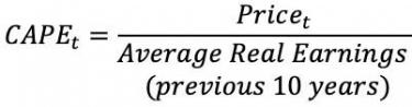
CAPE was designed as a measure of irrational bubbles (see Statman (2018) for an excellent discussion). The standard PE ratio gives a measure of the valuation of an asset, and CAPE simply grounds that measure with some recent-historical perspective in the form of earnings averaging. CAPE has historically been used to examine the valuation of the U.S. equity market as a whole (usually proxied by the S&P 500), although the measure has been extended to evaluate other assets as well. Investors’ willingness to tolerate expensive assets is, to some extent, a function of their risk aversion. Investors tend to become less risk averse near the end of bull market cycles, bidding up prices, and therefore facilitating lower future returns. The mean reversion of these valuations induces the predictability of long-run returns.

Importantly, CAPE was not designed to be a market-timing mechanism. When applied to the U.S. aggregate stock market by computing it for the S&P 500, it has been demonstrated to forecast market returns over the next 10 years. There is no assertion about the sequence of market returns to achieve that forecast—returns could be very high over the first five years, followed by very low returns the next five, or vice-versa, or any of an infinite number of combinations. Given the importance of sequence-of-return risk in many financial planning contexts, this provides a ceiling on the usefulness of the measure (albeit a high one).

Using data from the Federal Reserve’s Financial Accounts of the United States (abbreviated Z.1), it is possible to easily construct RISK, an estimate of the percentage of risky assets that household and nonprofit investors hold relative to their overall invested assets. Define this variable as:

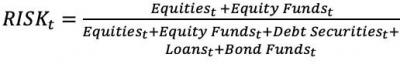
The details of the construction of this ratio are provided in Appendix A, but importantly, all variables are the nominal dollar-value holdings of the stated security classes by households and nonprofit entities (which are lumped together in data reporting by the Federal Reserve). For example, “Equities” is the total holding of equities by U.S. households and nonprofit entities.

Studies such as Kumar and Lee (2006) find evidence suggesting that retail stock trading may be reflective of sentiment rather than fundamentals, and that a given retail investor’s behavior is positively correlated with other retail investors. This suggests that times in which households increase their risky holdings are likely to be times of increasing prices for risky assets that are followed by below-average market returns. In this way, RISK may be a proxy for a behavioral irrationality on the part of household investors, but one that captures these investment errors in a different way than CAPE.³

To examine the forecasting ability of CAPE and RISK, this study collects data for the two measures over the entire time period for which both measures can be constructed. The Z.1 report has been published quarterly since 1951, and annual data is available back to 1946. The RISK variable is constructed with an annual frequency beginning in 1946. Specifically, because Z.1 is published with a lag while the data is collected, in years 1951 and forward RISK is computed in year t using third quarter data from year t-1. For 1945–1951, the annual data from the beginning of the year is used, which is the earliest availability.

CAPE is available as a longer series. Shiller provides the series monthly back to 1881, and this study collects CAPE from that series.⁴  For this examination, CAPE from December of year t-1 is used in year t to ensure availability to investors, similar to the construction of RISK above. To match the availability of RISK, CAPE is constructed as an annual series since 1946.

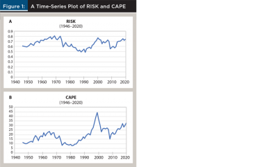
Figure 1 provides a time-series plot of RISK (in Panel A) and CAPE (in Panel B), while descriptive statistics for the two series may be seen in Table 1. The two series are clearly positively correlated (Table 1 indicates that this correlation is 0.383) but also are clearly capturing different phenomenon. For example, CAPE reaches a nadir in this time period in 1981 with a value of 7.83, while RISK that year is not far from its mean, around 0.65. In 1991, RISK reaches its low point of 0.49, while CAPE at the time is around 15.84. The scatterplot in Figure 2 serves to provide an intuitive illustration of the imperfect correlation between the two series.

 

 

 

 

 

 

 

 

 

 

 

 

Forecasting Comparison: CAPE Versus RISK

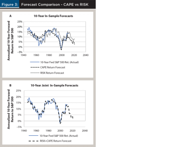
For three decades, CAPE has been studied and demonstrated to be an effective forecaster of long-term aggregate stock market returns.⁵  As such, it has been of use to financial planners in portfolio construction (informing expected returns) and in long-range planning (Blanchett 2015). Figure 3 Panel A provides a comparison of 10-year ahead annualized in-sample forecasts of S&P 500 returns generated from CAPE and RISK from 1946–2020 with the actual 10-year forward returns.⁶  Actual returns are only illustrated until 2010 since that is the last year for which such return can be constructed. Upon casual inspection, both CAPE and RISK appear to provide roughly similar-quality forecasts. However, the CAPE forecast is quantifiably better, explaining 66 percent of the variation in the series, compared to about 50 percent of the variation explained by RISK.

In Figure 3 Panel B, however, notice that the use of both variables jointly provides a much better forecast than either variable alone. The joint CAPE-RISK forecast explains a striking 87 percent of the variation in the series.⁷  Even visually, the improved quality of the forecast is evident. Combined use of RISK and CAPE have the potential to significantly improve financial planning tasks in which forecasts of long-term future market conditions are required.

 

 

 

 

CAPE is considerably less useful in forecasting short-term market returns (for the purposes of this study, “short-term” has been defined as one year ahead). In forecasts similar to those examined in Figure 3, CAPE forecasts explain less than 7 percent of the variation of one-year ahead S&P 500 returns in-sample. By comparison, RISK forecasts explain a bit more than 11 percent of the variation. This is still quite noisy, but almost twice the explained variation as CAPE. This can be seen visually in Figure 4 Panels A and B, which provide scatterplots of the one-year forward S&P 500 returns compared with CAPE and RISK, respectively. The better organized plot in Panel B is evident.

 

 

 

 

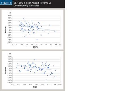
These scatterplots indicate the usefulness of RISK as an indicator relative to CAPE. In the 10 years when CAPE is above 27.45 (one standard deviation above its mean), the average return to the S&P 500 the following year was 10.04 percent. In the 13 years when RISK is above 0.742 (one standard deviation above its mean), the average return to the S&P 500 the following year was 1.36 percent. RISK provides a better short-term “dashboard” risk indicator than CAPE.

Crucially, RISK outperforms CAPE’s short-term forecasting performance to an even greater degree in out-of-sample tests. In a regression test that establishes an expanding window of regressions (so that only information available at time t-1 is used to forecast returns at time t), the mean square error (MSE) of the forecasts for RISK is 0.023. The corresponding MSE for CAPE is 0.028, implying the forecasting error for RISK is almost 20 percent lower than for CAPE. Even more telling, just using the past mean of the return series as the forecast yields an MSE of 0.026. Stated more clearly, the financial planner is better off just using the average returns as the forecast than he or she is using CAPE. Unfortunately, using CAPE and RISK together in the forecast is not as good as using RISK alone, yielding an MSE of 0.025.⁸

A RISK-Based Dynamic Allocation Strategy Example

The outperformance of RISK relative to CAPE for short-term forecasting can imply notable improvements in the financial planning process if properly employed. For example, Kitces and Pfau (2015), in articulating the case for dynamic glide paths (including CAPE-dependent glide paths) for retiree asset allocations, chose annual portfolio rebalancing in their analysis, following Bengen (1994). This study considers here an example of a static asset allocation application of Bengen’s seminal paper compared to two different conditional dynamic asset allocation glide paths—one conditional on CAPE, the other on RISK.

Following Bengen (1994), this study conducts a historical simulation using overlapping periods for which a 30-year retirement may be evaluated. Because RISK is only available beginning in 1946, this analysis will begin that year. Further, to ensure proper out-of-sample estimation, the first 15 years of RISK and CAPE are used as an initial estimation window, meaning the first year for evaluation will be 1961. The final year for which the outcome of a 30-year retirement can be determined is 1990 (since the data in this study extends through 2020). The example here has the drawback of being a bit shorter than is the typical interval for these types of studies, notably excluding the Great Depression years. However, the purpose of this study is to illustrate the benefit of utilizing RISK in financial planning situations, not to provide a comprehensive test of this particular retirement strategy.

The data for the example comes from several sources. Inflation rates, CAPE, and the prices and dividends for the S&P 500 (which are used to construct equity market returns) are collected from Robert Shiller’s website, as cited above. For bond returns, this study uses the Long-Term Corporate Bond series from Ibbotson SBBI Yearbook 2017: Stocks, Bonds, Bills and Inflation 1926–2016. For years 2017–2020, this series is augmented with returns to the Bloomberg-Barclays Aggregate Bond Total Return Index, collected from Bloomberg ticker symbol LBUSTRUU Index. The RISK variable as defined above is constructed from series in the Financial Accounts of the United States (Z.1).

The base case will follow the Bengen (1994) approach. In a given year, assume a retiree begins with $100 in retirement savings and a fixed portfolio allocation between stocks and bonds, and establishes a withdrawal rate the first year. Each year thereafter over the sample period, the withdrawal is adjusted by the inflation rate. For a range of asset allocations and initial withdrawal rates, Table 2 provides the median concluding wealth (discounted to the retirement year by the rate of inflation) of the strategy in Panel A, along with the minimum duration that the portfolio lasted in years in Panel B. These numbers naturally deviate from Bengen (1994), as this study begins in 1961 and uses data through 2020, essentially rolling his sample forward about 30 years. SAFEMAX, reported in Panel C, provides the highest withdrawal rate for the portfolio allocation that results in zero years in which the retirement portfolio is exhausted.

 

 

 

 

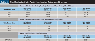
The commonly noted phenomenon that stock-heavier portfolios tend to be “safer” in the sense that they yield greater terminal wealth and a higher minimum number of years that the retirement portfolio may last for a given withdrawal rate can be seen in the table. Accordingly, SAFEMAX increases with the allocation to stocks.

To compare the potential effects of the CAPE and RISK variables on this approach, this study develops a dynamic asset allocation strategy based on stock return forecasts from each of these two variables. For each year, the relationship between the variable and forward stock returns is estimated (via regression) using data from all preceding years. Then, given the current state of the variable, the estimated regression is used to provide a forecast for the stock market over the following year. If the forecast is greater than a designated threshold, the default asset allocation is used. If the forecast falls below the threshold, a defensive asset allocation is assumed. For this example, we arbitrarily choose a return threshold of 10 percent and a defensive asset allocation of 30 percent stocks and 70 percent bonds.⁹

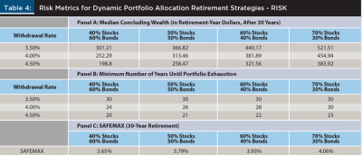
The experiment from the static asset allocation is repeated here, save for the adjustments to incorporate the dynamic asset allocation for both CAPE and RISK. The results are provided in Tables 3 and 4. The benefit of conditioning the portfolio allocation on the RISK forecast is evident. For every default asset allocation and withdrawal rate combination, the RISK-based dynamic portfolio strategy provided a higher median concluding wealth and lasted at least as long as the static portfolio allocation. SAFEMAX was equal to or higher than the static allocation in all cases.

 

 

 

 

 

 

 

 

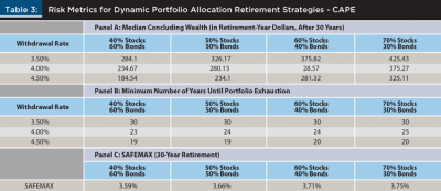
The performance of the CAPE-based forecast strategy was mixed. For more aggressive portfolio allocations, the median concluding wealth of these dynamic strategies tended to be greater than the static allocation. However, for the less stock-heavy allocations, the static strategy tended to outperform the CAPE-based strategy, both in median concluding wealth and the minimum number of years the portfolio lasted. In every case, the CAPE-derived strategy underperformed the RISK-derived one. This middling performance of the CAPE-derived strategy is surprising given the long-established association between CAPE and subsequent stock market returns. However, it is not terribly surprising given the findings in the previous section. CAPE is very effective in describing long-term asset returns, but much less so in describing stock market returns over a one-year horizon. Dynamic retirement asset allocations require implicitly making repeated short-term market forecasts—in this example, at a one-year horizon.

These middling results may also be a consequence of any one of a number of other drivers: the limited time horizon of this example (only the post-WWII period is included), the particular threshold chosen for swapping into a defensive portfolio, or the particular defensive asset allocation. None of these variables have been optimized. But neither were they optimized for the RISK-derived strategies, which yields the ultimate point of this study: the greater association of RISK with short-horizon future market returns relative to CAPE, coupled with the different behavioral phenomena it captures, provides a distinct advantage to the financial planner of considering the RISK variable as part of the decision-making process. The point is not to discount the value of CAPE, but rather to demonstrate the added benefit of considering RISK.

A Simple Example of Putting RISK to Work

The previous section indicates that using RISK as part of a dynamic allocation strategy for a retiree may be able to increase their annual portfolio withdrawal rates, enhancing their quality of life. What would that look like “on the ground” for the retiree and the financial planner assisting them?

Consider a hypothetical situation of a recent retiree sitting down with her financial planner late in the day on March 31, 2021. The S&P 500 closed that day at 3,972.89. The retiree has $1 million in investable assets and a Social Security income of $30,000 annually. After a diligent determination, the financial planner determines the retiree to have a moderately aggressive risk tolerance, generally conducive to a 70/30 style portfolio.

A capable financial planner will tend to have a figurative “dashboard” of various indicators of market health at his or her disposal. For example, at the close of the day on March 31, the VIX stood at 19.40 while the 10-Year Treasury yield was 1.75 percent. These values indicate that the volatility in the market is similar to its long-run average and that interest rates are near long-term lows. The latter is naturally also an indication that bond returns are expected to be well below normal over the next few years.

Robert Shiller updates CAPE data for the S&P 500 frequently on his website, but on March 31 the most recently updated data would indicate that at the end of February, the S&P 500 price was 3883.43 implying a CAPE of 35.09.¹⁰  A diligent planner may update that value with the March 31 S&P 500 value, yielding an updated approximation of CAPE at 35.89. This is very high relative to the historical mean of CAPE since World War II, which is around 19.

Finally, the financial planner can update their estimate of RISK by accessing the five variables that define it, as described in the Appendix. Each value can be pulled directly from the website listed there. As of March 31, 2021, the five variables had been last updated in publication Z.1 by the Federal Reserve on March 11. The values are: equities, $24,719,070; equity funds, $7,728,892; debt securities, $5,077,050; loans, $1,024,680; and bond funds, $3,172,346 (these values are all in millions, but because this is true for all five variables, it is not necessary to make any adjustments in the ratio below).

With RISK defined as above, the values imply that on March 31, 2021:

It is of note that this value is not far from the all-time high of this series of 0.807 in 1969. In the previous section, we demonstrated that a dynamic asset allocation for retirees in which they take a defensive position when RISK is sufficiently high can justify higher withdrawal rates.

Assume that the financial planner takes the dynamic asset allocation strategy of the previous section to heart, even if their response is not quite as mechanical as the situation described there. With RISK at this level, the financial planner may want to seriously consider a defensive allocation, and the high reading of CAPE only serves to reinforce the need for such consideration. Following the RISK-based dynamic allocation strategy in Table 4, the financial planner decides that the defensive allocation of 30/70 is appropriate for this year, and that a 70/30 portfolio will be the default moving forward, in line with the client’s risk profile.

Referencing SAFEMAX in Table 4, the financial planner decides that a 4 percent withdrawal rate is appropriate. This implies that an investment derived income of $40,000 can be matched with the client’s $30,000 Social Security income, implying an annual real budget for the client of $70,000 moving forward.

Implications for Financial Planners

Behavioral variables have been demonstrated to provide important insight into the current market environment, and some systematic behavioral tendencies of market participants have been shown to induce a degree of predictability in asset markets. This predictability does not imply the ability to reliably time the market, but it does imply the ability to gauge fluctuating market environments and tilt client portfolios—or simply manage client expectations—accordingly. Dynamic glide paths conditional on CAPE (Kitces and Pfau 2015) are one example of such tilts, while ascertaining the probability of market success as a function of CAPE (Blanchett 2015) is another. But these are only two potential applications; there are many more.

Variables that are informative enough for a financial planner to get a read on the market environment are relatively rare. The VIX, Treasury yields, the USD/EUR exchange rate, etc., are part of the figurative dashboard regularly monitored by financial planners practicing their fiduciary responsibility.

CAPE has gradually, and rightly, become the first behavioral variable to merit inclusion in this instrumentation. RISK captures the behavioral environment from a different perspective than CAPE. Rather than a valuation lens, it provides a window into the asset allocation decisions of households. This is important, as academic research has demonstrated that retail investors exhibit systematic shortcomings in their investment selections. Accordingly, this study has presented strong evidence that RISK is negatively related to subsequent aggregate stock market movements. As such, it can provide another potential warning light to financial planners, and it can potentially do so during times even in which CAPE provides a reading that is somewhat benign. 

Endnotes

1. Similar ratios have also been developed in unpublished work by Zhang (2014) and Yan and Zhang (2017). Those two works use slightly different implementations that are highly correlated with the RISK variable presented here, the latter of which aligns closely with the definition in this study and is an excellent reference for a rigorous treatment of the forecasting properties of RISK.
2. In the later work, this variable is denoted by the more cumbersome moniker P/Ten Year MA(E).
3. A prominent example of academic work suggesting this relationship is Baker and Wurgler (2000), who study the share of total new security issues as equity relative to debt, calculated from data reported in the Federal Reserve Bulletin (the key difference between their measure and ours is that they look not at total asset holdings, but rather only new issues).
4. The series is available publicly at www.econ.yale.edu/~shiller/data.htm under the link “U.S. Stock Markets 1871-Present and CAPE Ratio.”
5. A detailed look at the forecasting properties of CAPE is beyond the scope of this study. Philips and Ural (2016) provide an excellent place to start for an examination of those properties. Since the forecasting properties of CAPE are so well established, this study focuses on in-sample forecasts in the exposition for the sake of clarity.
6. Forecasts in Figure 3, Panel A come from two OLS regressions of 10-year ahead S&P 500 returns (separately) on CAPE and RISK. The resulting estimated equation for the CAPE forecast is: 10-year ahead S&P 500 Return = 0.209-0.005*CAPE. The resulting estimated equation for the RISK forecast is: 10-year ahead S&P 500 Return = 0.400-0.443*RISK. All coefficients in both equations are significant at the 1 percent level, adjusting for heteroskedasticity. The R² for each regression is 0.66 and 0.50, respectively.
7. Forecasts in Figure 3, Panel B come from an OLS regression of 10-year ahead S&P 500 returns on CAPE and RISK jointly. The resulting estimated equation for the forecast is: 10-year ahead S&P 500 Return = 0.389-0.004*CAPE-0.305*RISK. All coefficients in the equation are significant at the 1 percent level, adjusting for heteroskedasticity. The R² for the regression is 0.87.
8. With noisy models such as these, it is often the case that models with greater numbers of parameters underperform more parsimonious models out-of-sample. The reason for this is the uncertainty of the parameter estimates accumulate, which induces error in the out-of-sample forecasts.
9. Naturally, these values may be adjusted. These were chosen as they were reasonable values for this illustrative example.
10. Verification of these values and the spreadsheet with the functions to carry out this analysis may be found at www.econ.yale.edu/~shiller/data.htm under the link “U.S. Stock Markets 1871-Present and CAPE Ratio.”

References

Baker, Malcolm, and Jeffrey Wurgler. 2000. “The Equity Share in New Issues and Aggregate Stock Returns.” Journal of Finance 55: 2,219–2,257.

Bengen, William P. 1994. “Determining Withdrawal Rates Using Historical Data.” Journal of Financial Planning 7 (4): 171–180.

Blanchett, David M. 2015. “Initial Conditions and Optimal Retirement Glide Paths.” Journal of Financial Planning 28 (9): 52–60.

Campbell, John Y., and Robert J. Shiller. 1998. “Valuation Ratios and the Long-Run Stock Market Outlook.” Journal of Portfolio Management 24 (2) 11–26.

Campbell, John Y., and Robert J. Shiller. 1988. “Stock Prices, Earnings and Expected Dividends.” Journal of Finance 43 (3) 661–676.

Ibbotson, Roger. 2017. 2017 SBBI Yearbook: Stocks, Bonds, Bills and Inflation. Hoboken, N.J.: John Wiley & Sons.

Kitces, Michael E. and Wade D. Pfau. 2015. “Retirement Risk, Rising Equity Glide Paths, and Valuation-Based Asset Allocation.” Journal of Financial Planning 28 (3): 38–48.

Kumar, Alok, and Charles M.C. Lee.2006. “Retail Investor Sentiment and Return Comovements.” Journal of Finance 61 (5) 2,451–2,486.

Philips, Thomas, and Cenk Ural. 2016. “Uncloaking Campbell and Shiller’s CAPE: A Comprehensive Guide to Its Construction and Use.” Journal of Portfolio Management 43 (1): 109–125.

Radha, Sailesh S. 2020. “Using CAPE to Forecast Country Returns for Designing an International Country Rotation Portfolio.” Journal of Portfolio Management 46 (7): 101–117.

Shiller, Robert. 2005. Irrational Exuberance. Princeton, N.J.: Princeton University Press.

Statman, Meir. 2018. “Behavioral Efficient Markets.” Journal of Portfolio Management 44 (3): 76–87.

Welch, Ivo, and Amit Goyal. 2007. “A Comprehensive Look at The Empirical Performance of Equity Premium Prediction.” Review of Financial Studies 21 (4): 1,455–1,508.

Yan, David C., and Fan Zhang. 2017. “Be Fearful When Households are Greedy: The Household Equity Share and Expected Market Returns.” SSRN Working Paper no. 3034548.

Zhang, F. (2014) “Essays in Financial Economics.” Doctoral Dissertation, Harvard University. Available at dash.harvard.edu/handle/1/12274634.

Citation

Fink, Jason, and Kristin Fink. 2021. “The RISK that Households Take: A Behavioral Variable Worth Watching.” Journal of Financial Planning 34 (7): 84–95.

 

Appendix A: Construction RISK from Publicly Available Data

Data for the calculation of RISK is collected from the Federal Reserve Financial Accounts of the United States (release Z.1), which is published quarterly by the Federal Government, and may be found online at federalreserve.gov/releases/z1/. From that page, it is possible to download the most recent publication in a single .pdf file or to pull data as .csv files (in zipped form). It is also possible (and most straightforward) to download the values and their history from the FRED Economic Database of the St. Louis Federal Reserve. The specific web pages for the data will be listed with each series below.

    RISK is defined as:

All variables are the nominal dollar-value holdings of the stated security classes by households and nonprofit entities. Each variable is defined and may be collected as follows:

Equities_t: Households and Nonprofit Organizations, Corporate Equities, Asset, Level. This can be collected from line 15 in Table B.101.e of the Z.1 release. Alternatively, it may be found as series HNOCEAQ027S in the Fred database, and downloaded directly from alfred.stlouisfed.org/series?seid=HNOCEAQ027S.

Equity Funds_t: Households and Nonprofit Organizations, Mutual Fund Shares, Equity Funds; Asset, Level. This can be collected from line 21 in Table B.101.e of the Z.1 release. Alternatively, it may be found as series BOGZ1FL153064245Q in the Fred database, and downloaded directly from alfred.stlouisfed.org/series?seid=BOGZ1FL153064245Q.

Debt Securities_t: Households and Nonprofit Organizations, Debt Securities, Asset, Level. This can be collected from line 6 in Table L.101 of the Z.1 release. Alternatively, it may be found as series HNODSAQ027S in the Fred database, and downloaded directly from alfred.stlouisfed.org/series?seid=HNODSAQ027S.

Loans_t: Households and Nonprofit Organizations, Loans, Asset, Level. This can be collected from line 30 in Table L.214 of the Z.1 release. Alternatively, it may be found as series HNOLA in the Fred database, and downloaded directly from alfred.stlouisfed.org/series?seid=HNOLA.

Bond Funds_t: Households and Nonprofit Organizations, Mutual Fund Shares, Bond Funds. This can be collected from line 4 in Table 7HH of the Z.1 release. Alternatively, it may be found as series BOGZ1FL153064235Q in the Fred database, and downloaded directly from alfred.stlouisfed.orgseries?seid=BOGZ1FL153064235Q.