Journal of Financial Planning: September 2015
David M. Blanchett, CFP®, CFA, is head of retirement research at Morningstar Investment Management. He is the 2015 recipient of the Journal’s Montgomery-Warschauer Award for his May 2014 Journal paper “Exploring the Retirement Consumption Puzzle.”
Executive Summary
- Traditional financial planning theory generally suggests that a retirement glide path should become more conservative as an individual ages.
- Using a model based on long-term averages or one that does not take into account initial conditions for both stocks and bonds can lead to misleading conclusions about the optimal glide path shape for retirees today.
- This paper introduces a return model that incorporates varying levels of initial bond yields and stock market valuations.
- Increasing glide paths appear to perform best in higher-return environments, while decreasing glide paths perform better in lower-return environments.
- Based on current market conditions, decreasing glide paths result in a slightly higher probability of success for a retiree when compared to a constant or increasing glide path with the same general level of risk in retirement.
The body of research exploring the optimal glide path shape for investors, both for accumulation and distribution phases of retirement, continues to grow. Traditional financial planning theory generally suggests that the retirement glide path should include an equity allocation approximating 100 percent minus an investor’s age. For example, a 30-year-old should have 70 percent in stocks, and a 70-year-old should hold 30 percent in stocks.
Different approaches exist, but the optimal glide path shape is commonly assumed to decrease throughout someone’s lifetime, meaning the portfolio should become more conservative as the individual approaches retirement. Both Basu and Drew (2009) and Arnott, Sherrerd, and Wu (2013) have demonstrated that an inverse glide path results in more wealth, on average, for potential retirees. The theory behind a decreasing glide path is consistent with the Bodie, Merton, and Samuelson (1992) model in which the bond-like labor income portion of a household total wealth portfolio falls with age and is replaced with actual bonds from financial markets. This explains why no target date mutual fund provides an increasing glide path.
Retirement experts have mostly agreed on a decreasing optimal glide path until recently. Although past researchers, such as Cocco, Gomes, and Maenhout (2005) and Gomes, Kotlikoff, and Viceira (2008), have noted a rising glide path may be best for retirees, it was not until research by Pfau and Kitces (2014)—which also noted the potential benefit of an increasing retiree glide path—that many financial planners started questioning the optimal glide path shape. Using four metrics, such as the probability of success and the magnitude of failure, Pfau and Kitces noted a slight improvement in the probability of success by using an increasing glide path (generally +/–3 percent for similar risk levels).
Blanchett (2015) reached the opposite conclusion, determining that declining glide paths are optimal. Blanchett’s approach was different than the method used by Pfau and Kitces: he tested more scenarios, used a utility model to incorporate preferences, and evaluated different glide path shapes. However, as this paper will demonstrate, a key reason for the differences in findings between Blanchett (2015) and Pfau and Kitces (2014) was the return assumptions used. Blanchett based his analysis on a model that incorporated today’s low bond yields, where the yields were assumed to slowly increase, on average, throughout retirement. Blanchett’s research was an update on a 2007 study in which static glide paths were generally noted to be optimal; however, rising glide paths were not considered.
In another paper, Kitces and Pfau (2015) used a valuation-based asset allocation model based on the Shiller CAPE ratio. They found that although it is relatively difficult to beat a static 60 percent equity allocation during retirement (see Blanchett 2007), a rising glide path appears to provide potential downside risk protection for retirees in an overvalued stock market.
Although Blanchett (2015) incorporated today’s low yields, and Kitces and Pfau (2015) incorporated market valuation, neither research included both to determine the joint impact of retiring when the stock market is overvalued and interest rates are low. Understanding the implications of these initial conditions is the objective of this paper.
Market Conditions Today
Retirees need to consider both initial bond yields and stock market conditions at retirement. In this paper, two key indicators were used to forecast the future returns of bonds and stocks; namely, 10-year U.S. government bond yields and the Shiller CAPE ratio, respectively. Bond yields provide a great deal of insight to the future returns of bonds, because a majority of the return on bonds is the coupon, which is known at the time of purchase.
The CAPE ratio was introduced by Campbell and Shiller (1998) and is calculated by dividing the price level of the S&P 500 by the average real earnings over the previous 10 years. Campbell and Shiller noted that this metric can explain about 30 percent of subsequent real stock returns.
Research by Davis, Aliaga-Díaz, and Thomas (2012) also documented the historical predictive benefit of the CAPE ratio versus other common forecasting metrics. The historical relation between each of these metrics is included in Figure 1 for bonds and stocks. The bond data in Panel A is based on year-end yields and total returns for the Ibbotson Long-Term Government Bond Index series from 1926 to 2014. The stock return data in Panel B is the year-end CAPE Ratio and price return for the S&P 500 from 1881 to 2014 as published on Robert Shiller’s website.
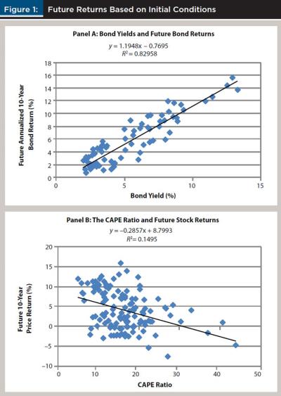
The relation between bond yields and future bond returns is much higher than the CAPE ratio and future stock returns; however, neither metric is favorable for retirees today, especially when compared to long-term averages. Kitces (2009) noted the relation between safe initial withdrawal rates based on various market valuation levels, whereby individuals who retire in an overvalued market should withdraw less initially than retirees who retire in an undervalued market.
Historically, the relation between bond yields and the CAPE ratio has been relatively minor, with a correlation of –0.13. This suggests that times of lower bond yields have generally been associated with times of higher CAPE ratios, but that the relation is very weak.
As of May 2015, the yield on 10-year U.S. Treasuries was 2.12 percent. The CAPE ratio was approximately 27.5. To provide some perspective about how extreme the current values are today, only six of the last 135 years (as of January 1) had yields lower than 2.25 percent, and only six of the past 135 years had a CAPE ratio above 27. Understanding where things are today is very important, because today’s conditions will likely have a significant impact on retiree outcomes.
Retirement researchers commonly use long-term historical return averages, with the most popular data set being the Ibbotson time series for stocks, bonds, Treasury bills, and inflation (SBBI) going back to 1926. Although this historical series may seem significant, it is less meaningful given the current market environment. For example, the average historical yield on 10-year Treasury bonds since 1881 has been 4.5 percent. The current yield on 10-year Treasury bonds is less than half the long-term average. Therefore, an analysis based on long-term averages makes the implicit assumption that an investor can purchase 10-year government bonds that will yield 4.5 percent, on average, despite the fact it is impossible to obtain such yields today.
The safety of an initial withdrawal rate, as well as conclusions about the optimal glide path, is heavily dependent on the return assumptions used in the model. For example, the safety of Bengen’s (1994) initial 4 percent rule changes considerably when a financial planner uses return expectations better calibrated to current market conditions. This is especially true because the returns experienced early in retirement have a disproportional weight on the outcome of the retirement scenario, a concept commonly referred to as sequence risk. In order to achieve the same approximate probabilities of success using historical data to determine the 4 percent rule would result in a 3 percent rule today.
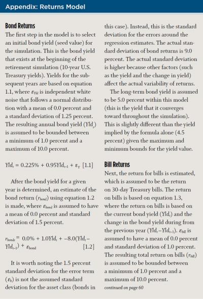
Returns Model
The returns model used in this paper is an updated version of an approach introduced by Blanchett, Finke, and Pfau (2014; 2015). The returns model is based on the general relations noted in Figure 1, whereby lower bond yields tend to correlate to lower bond returns and higher CAPE ratios tend to correlate to lower stock returns. The model begins with two separate assumptions: the interest rate upon retirement and the CAPE ratio upon retirement. The appendix on page 59 provides more specific information about the model.
The initial interest rate (the interest rate seed), is the yield on 10-year Treasury bonds upon retirement. The base assumption is that the yield converges back to its long-term average over time, which is assumed to be 5 percent. Therefore, if retirement is assumed to begin in a low-yield environment the yield will increase each year. The low yield has a dual effect on the bond returns. The assumed yield return (income return) is lower, and the price return (change in value of the portfolio) may be negative because the return on bonds is inversely correlated to changes in bond yields.
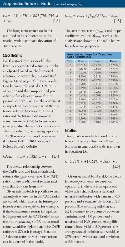
The equilibrium CAPE value is assumed to be 17, which is close to the long-term average. With a CAPE value of 17, the arithmetic average return on stocks in the model is approximately 9 percent with an annualized standard deviation of 18 percent. To be more consistent with equity returns in international markets, the expected return on stocks is lower than the actual historical long-term return on stocks. The long-term compounded average annual return of U.S. equities has averaged about 2 percentage points higher than the other 20 countries in the Dimson-Marsh-Staunton dataset, which goes back to 1900 (data were obtained from Morningstar Direct and adjusted accordingly).
Historically, higher CAPE values have been associated with lower returns, and vice-a-versa. The model used in this analysis incorporates this historical relation for the first 15 years of retirement. For example, if the CAPE ratio is higher than average (above 17), the returns on equities will be lower than average; and if the CAPE ratio is below average, the returns will be higher than average.
Additionally, an investment fee of 50 basis points is included in the simulations. The fee is included to reflect the fact that it is impossible to invest for free. Although it is possible to build a portfolio of index mutual funds or ETFs at a relatively low cost, the average investor typically pays more when investing, either through actively managed investments, investment advisory fees, or both.
Figure 2 provides some perspective on how changing key assumptions can affect the probability of a portfolio being able to successfully fund a 4 percent initial withdrawal rate over a 30-year retirement period for varying equity allocations (from 0 percent to 100 percent equities in 10 percent increments). The initial withdrawal amount, which is 4 percent of the initial balance of the portfolio, is assumed to increase annually by inflation. The results illustrated in Figure 2 are based on the model using a 10,000-run Monte Carlo simulation.
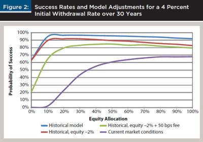
Three key assumptions underlie the historical returns model in Figure 2 (the top blue line). The first is a reduction in the assumed rate of return of equities by 2 percent to better reflect the average historical returns in equities internationally. The second is the inclusion of a 50 basis point fee in the portfolio, and the third is to assume that an individual retires in an environment similar to today, where the initial yield on bonds is assumed to be 2.5 percent and the CAPE ratio is assumed to be 27.
Figure 2 provides powerful evidence that although 4 percent was a relatively safe initial withdrawal rate historically, it is considerably less safe today, having a probability of success of approximately 50 percent for a balanced portfolios based on today’s market conditions.
Analysis
Three primary glide path shapes were considered for the analysis: decreasing, constant, and increasing. The decreasing glide path had an initial allocation of 60 percent equities that decreased by 1 percent each year during retirement. The constant glide path had a 45 percent equity allocation constant throughout retirement. The increasing glide path had an initial equity allocation of 30 percent that increased 1 percent per year in retirement. Each glide path was created as a relatively balanced portfolio during retirement, where the average allocation over a 30-year retirement period was equal to the constant glide path.
The fixed income portion of the portfolio was assumed to be 75 percent bonds and 25 percent Treasury bills. Note that the results are not sensitive to this assumption and are effectively the same if these weights are reversed (additional information regarding the impact of the allocation to bills is addressed in a future section).
Three initial CAPE ratios were tested (10, 17, and 27). Three bond yield seeds were considered (2.5 percent, 5.0 percent, and 7.5 percent). The initial withdrawal rate was assumed to be 4 percent for this test, although this assumption was varied in future tests. The subsequent portfolio withdrawals were assumed to increase annually with inflation, which is consistent with the assumptions used to determine the 4 percent rule. The retirement period was assumed to last 30 years for this test, although varied for future tests. Taxes were ignored for the analysis.
Table 1 includes information about the optimal respective glide path shape for the nine different base test scenarios, as well as the respective probabilities of success for each (in relative order from best to worst).
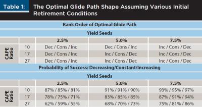
The results in Table 1 demonstrate a few things. On average, the increasing glide path is optimal for moderate- or high-yield seeds, while the decreasing glide path is optimal for low-yield scenarios. If a financial planner focuses on both “moderate” scenarios (yield seed of 5 percent and an initial CAPE ratio of 17), the increasing glide path is best (with an 85 percent success rate), while the decreasing glide path is worst (83 percent).
The return assumptions significantly affect both the optimal glide path shape as well as the relative safety of the initial withdrawal rate. Depending on whether a financial planner assumes initial bond yields are low or high can significantly impact the definition of optimal (the order can reverse). Also, the initial yield seeds tend to impact the order of the results more than the initial CAPE ratio.
Regardless of the scenario, the differences across the glide paths (increasing versus decreasing) really are not all that different. For example, among the nine scenarios, the one that is most similar to conditions today is the one with an initial yield seed of 2.5 percent and a CAPE ratio of 27. Under these assumptions, the optimal glide path shape is decreasing, followed by constant. An increasing glide path is the worst, with probabilities of success of 62 percent, 59 percent, and 55 percent, respectively. Although the difference between the best glide path shape (decreasing) and worst glide path shape (increasing) may seem material, these are not really economically significant, as there is not a material change in the outcome for a retiree.
For example, an important assumption in retirement modeling is the length of retirement period. Using a 30-year retirement period is a common assumption, however there is only approximately a 5 percent chance that the retirement period for a married couple, male and female both age 65, will end in the 30th year of retirement. In reality, the retirement period will likely be shorter or longer than 30 years. As the expected duration of retirement changes, so too does the relative potential benefit of the different glide path shapes.
Table 2 includes the probabilities of success for a 4 percent initial withdrawal rate for the nine base scenarios included in Table 1. The table also includes retirement periods lasting 20, 25, 30, 35, and 40 years. Current markets are highlighted in yellow.
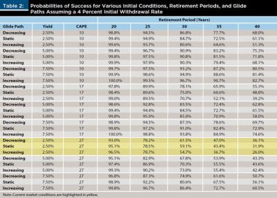
The optimal glide path shape changes considerably based on potential length of retirement. The increasing glide path is generally optimal for the simulations with higher probabilities of success, such as the 20-year simulations, but the relative level of optimality changes based on the assumed base assumptions.
One important assumption that was not varied is initial withdrawal rate. Although a 4 percent initial withdrawal rate is popular in the retirement planning literature, the results of these simulations—using today’s market conditions—suggest that this rule is much less safe than historical estimates would suggest. Therefore, it is important to understand how the results would potentially change as initial withdrawal rates and retirement periods are varied. These results are included in Table 3, where the assumed initial values are based on today’s initial conditions, with a CAPE ratio of 27 and a bond yield seed of 2.5 percent.
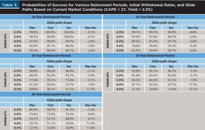
Table 3 also provides important insights. First, a 3 percent initial withdrawal rate over 30 years, based on today’s market conditions, results in the same approximate probability of success as a 4 percent initial withdrawal rate based on historical long-term averages.
Consistent with results in Tables 1 and 2, the increasing glide path results in higher probabilities of success for the safer simulations, such as a 3 percent initial withdrawal rate. An important consideration is exactly how risk is defined. The increasing glide path tends to be optimal when there is a relatively higher probability of success or when the likelihood of a bad outcome is low. The decreasing glide paths tend to do better when the probabilities of success decrease, particularly if the retiree lives longer than expected or needs a higher withdrawal rate. Therefore, if a financial planner is designing a glide path to protect against the worst-case scenario, the decreasing glide path may be considered a better hedge.
The Treasury Bill Situation
The base assumption for this analysis was that Treasury bills represented 25 percent of the fixed income allocation. In order to determine the relative impact of different Treasury bill allocations, an analysis was conducted where the allocations to bills was varied. The analysis varied the allocation to bills from 0 percent to 100 percent of the non-equity allocation, in 10 percent increments. The simulations were based on current market conditions and both 3 percent and 4 percent initial withdrawal rates were tested. The results of the simulations are included in Table 4.
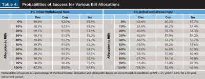
The values in Table 4 suggest that higher allocations to Treasury bills lead to lower probabilities of success, on average, regardless of the glide path shape. The impact is most significant for the 4 percent initial withdrawal rate (where the probabilities of success are lower). One important assumption for this analysis is that the allocations to Treasury bills (as a portion of the fixed income allocation) are held constant for the duration of retirement. In reality, a retiree may choose to allocate relatively more to Treasury bills today and move into bonds after interest rates have increased.
Additional Considerations
This paper raises a number of important implications for financial planners. First, as noted previously in a number of research projects by Blanchett, Finke, and Pfau (2013; 2014; 2015), using a model based on expected returns results in a very different estimate of the probability of success for a 4 percent initial withdrawal rate over a 30-year retirement period compared with a model based on historical returns. This does not mean that a 4 percent initial withdrawal rate (or more) cannot still work given the nuances associated with implementation. For example, most retirees will not need to spend the same amount each year (in real terms) during retirement. Retirees can adjust consumption based on portfolio performance, and even if the portfolio were to fail, most retirees would not be truly destitute given governmental support programs like Social Security. Also, probability of success is only one way to measure an outcome for a retiree. This measure of success does not incorporate important considerations like the magnitude of failure.
In terms of optimal retiree glide path shape, the best glide path is heavily dependent on model assumptions, such as how long the retiree is going to live and the returns the retiree is likely to achieve during retirement. Using long-term averages tends to suggest that an increasing glide path may be best, but using a model that is better calibrated to today’s environment suggests a decreasing glide path may optimal for investors living 30 years or longer past initial retirement. Overall, the differences among glide paths with similar lifetime risk levels are not really all that different and do not significantly change the outcomes for a retiree.
One impact variable that is not considered in this analysis that is important to retirees is risk tolerance or risk preference. As a retirees age, they tend to prefer more conservative portfolios. It is difficult to incorporate risk tolerance into common retirement income planning models because models are largely focused on accomplishing a goal. However, if risk preference were directly incorporated into models, it would likely provide an additional “nudge,” making decreasing glide paths more optimal than their more aggressive alternatives. This would be especially true if taking additional risk cannot be shown to produce more secure outcomes.
Conclusions
It is almost certain there will be more research on optimal glide paths in the future, both in accumulation and decumulation. This research should lead to more constructive conversations about what is the right portfolio for investors. Before accepting the conclusions of future research, it is important to understand the key assumptions of the models, as well as how changing assumptions may affect the results.
This study has demonstrated how initial market conditions can have a considerable impact on defining the optimal glide path shape. Using a model based on historical long-term averages indicates an increasing glide path may be optimal; however, a model that is better calibrated to today’s low yield and high valuation environment suggests that a decreasing glide path may be best for retirees, especially those with higher initial withdrawal rates or longer retirement periods. For more conservative retirees, especially those with a shorter retirement duration or lower initial withdrawal rate, an increasing glide path may be best, especially because it allows the retiree to begin retirement with a more conservative allocation and then potentially choose to take on more risk later in retirement.
Regardless of the glide path selected, the most relevant finding from this analysis is that initial portfolio withdrawal rates noted to be “safe” using historical averages, such as a 4 percent initial withdrawal, are more likely to result in a much higher probability of failure in the future. Also, the differences between the shapes are not that material, and other considerations, such as risk tolerance and retirement duration, are likely to materially affect the truly optimal glide path at the individual
retiree level.
References
Arnott, Robert D., Katrina F. Sherrerd, and Lillian J. Wu. 2013. “The Glidepath Illusion ... and Potential Solutions.” Journal of Retirement 1 (2): 13–28.
Basu, Anup K., and Michael E. Drew. 2009. “Portfolio Size Effect in Retirement Accounts: What Does It Imply for Lifecycle Asset Allocation Funds?” Journal of Portfolio Management (35) 3: 61–72.
Bengen, William P. 1994. “Determining Withdrawal Rates Using Historical Data.” Journal of Financial Planning 7 (4): 171–180.
Blanchett, David M. 2007. “Dynamic Allocation Strategies for Distribution Portfolios: Determining the Optimal Distribution Glide Path.” Journal of Financial Planning 20 (12): 68–81.
Blanchett, David M. 2015. “Revisiting the Optimal Distribution Glide Path.” Journal of Financial Planning 28 (2): 52–61.
Blanchett, David, Michael Finke, and Wade Pfau. 2013. “Low Bond Yields and Sustainable Withdrawal Rates.” Journal of Wealth Management 16 (2): 55–62.
Blanchett, David, Michael Finke, and Wade Pfau. 2014. “Asset Valuations and Safe Portfolio Withdrawal Rates” Retirement Management Journal 4 (1): 21–34.
Blanchett, David, Michael Finke, and Wade Pfau. 2015. “Retiring in a Low-Return Environment.” Advisor Perspectives Newsletter (April).
Bodie, Zvi, Robert C. Merton, and William F. Samuelson. 1992. “Labor Supply Flexibility and Portfolio Choice in a Life Cycle Model.” Journal of Economic Dynamics and Control 16 (3–4): 427–449.
Campbell, John Y., and Robert J. Shiller. 1998. “Valuation Ratios and the Long Run Stock Market Outlook.” Journal of Portfolio Management 24 (2): 11–26.
Cocco, Joao F., Francisco J. Gomes, and Pascal J. Maenhout. 2005. “Consumption and Portfolio Choice over the Life Cycle.” Review of Financial Studies 18 (2): 491–533.
Davis, Joseph, Roger Aliaga-Díaz, and Charles J. Thomas. 2012. “Forecasting Stock Returns: What Signals Matter, and What Do They Say Now?” Vanguard White Paper. personal.vanguard.com/pdf/s338.pdf.
Finke, Michael, Wade D. Pfau, and David M. Blanchett. 2013. “The 4 Percent Rule Is Not Safe in a Low-Yield World.” Journal of Financial Planning 26 (6): 46–55.
Gomes, Francisco J., Laurence J. Kotlikoff, and Luis M. Viceira. 2008. “Optimal Life-Cycle Investing with Flexible Labor Supply: A Welfare Analysis of Life-Cycle Funds.” American Economic Review 98 (2): 297–303.
Kitces, Michael E. 2009. “Dynamic Asset Allocation and Safe Withdrawal Rates.” The Kitces Report (April).
Kitces, Michael E., and Wade D. Pfau. 2015. “Retirement Risk, Rising Equity Glide Paths, and Valuation-Based Asset Allocation.” Journal of Financial Planning 28 (3): 38–48.
Pfau, Wade D., and Michael E. Kitces. 2014. “Reducing Retirement Risk with a Rising Equity Glide Path.” Journal of Financial Planning 27 (1): 38–45.
Citation
Blanchett, David M. 2015. “Initial Conditions and Optimal Retirement Glide Paths.” Journal of Financial Planning 28 (9): 52–60.