Journal of Financial Planning: May 2015
David Nanigian, Ph.D., is an associate professor of investments at The American College. He is internationally known for his research on mutual funds and regularly teaches a course on mutual funds in The American College’s Master of Science in Financial Services program. Learn more about his research at ssrn.com/author=843211.
The Capital Asset Pricing Model (CAPM), developed by William Sharpe and John Lintner, predicts that a stock’s return-generating process is characterized by the following form:
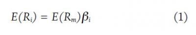
where E(Rm) is the expected return on the stock market in excess of the risk-free rate of interest, E(Ri) is the expected return on stock i in excess of the risk-free rate, and βi (beta) denotes
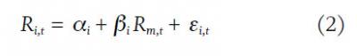
, i.e. the factor by which Ri comoves with Rm. βi is usually estimated through a univariate time-series regression of the following form:
Understanding the CAPM
The CAPM provides investors with a simple and intuitive model for how they should be compensated for bearing systematic risk, which affects the entire market and cannot be eliminated through diversification. The CAPM says that there is a one-to-one relationship between (1) the sensitivity of a stock’s excess return to variation in the excess return on the stock market; and (2) the expected return on the stock. It is also the predominant asset pricing model used by financial professionals.
For example, in a 2013 study (“Best Practices in Estimating the Cost of Capital: An Update,” published in the Journal of Applied Finance), Todd Brotherson, Kenneth Eades, Robert Harris, and Robert Higgins surveyed practitioners at leading companies and financial advisers on how they estimate the cost of capital. The authors found that 90 percent of the companies and 100 percent of the advisers in their sample relied solely on the CAPM in estimating a stock’s required return.
Similarly, in the Association for Financial Professionals’ 2013 Estimating and Applying Cost of Capital Survey, 85 percent of survey participants responded that they used the CAPM to estimate a stock’s required return. Perhaps it is because of this model’s preeminence that it is commonly referred to as “the Capital Asset Pricing Model” rather than the Sharpe-Lintner Capital Asset Pricing Model.
Despite the CAPM’s theoretical appeal and wide use in practice, it fails abysmally to predict returns. In a seminal 1992 Journal of Finance paper, “The Cross-Section of Expected Stock Returns,” Nobel Laureate Eugene Fama, along with Kenneth French, found that there was little relationship between beta and return. The results were confirmed in a subsequent 2014 paper (“Betting Against Beta” published in the Journal of Financial Economics) by Andrea Frazzini and Lasse Heje Pedersen that examined not only domestic stocks but also international stocks.
In a 2011 paper (“Benchmarks as Limits to Arbitrage: Understanding the Low-Volatility Anomaly,” published in the Financial Analysts Journal), Malcom Baker, Brendan Bradley, and Jeffrey Wurgler discovered a negative relationship between beta and return. The authors tracked the performance of five portfolios of stocks that were formed based on quintile rank of beta and reconstituted on a monthly basis. They found that the average excess return on the portfolio of stocks with the lowest betas was 5.07 percent, yet the average excess return on the portfolio of stocks with the highest betas was merely 1.53 percent.
To put this into perspective, consider an individual who invested $1 into the portfolio of stocks with the lowest betas and $1 into the portfolio of stocks with the highest betas in 1968. By 2008, the value of the portfolio of stocks with the lowest betas grew to $10.28 in real terms, while the value of the portfolio of stocks with the highest betas shrank to 64 cents in real terms.
At first blush, it may seem that investors would be well-advised to sell high beta stocks and buy low beta stocks. However, before employing any investment strategy one should always think deeply about the reasons for the performance of the strategy and draw upon those explanations to form a thesis on whether or not the performance will continue to persist. An irrational preference for high beta stocks, borrowing constraints, and tracking error volatility constraints are the three main explanations for the failure of the CAPM to predict returns. I discuss each of these in turn.
Why the CAPM Fails to Predict Returns
Contrary to the advice of a prudent financial planner, many people use the stock market to gamble. The stocks that offer the possibility of “hitting the jackpot”—typically technology stocks—tend to have high betas. Therefore, the existence of “gamblers” in the stock market creates greater demand for high beta stocks than for low beta stocks. This drags down the required return on high beta stocks to a lower level than that which is predicted by the CAPM, and pushes up the required return on low beta stocks to a higher level than that which is predicted by the CAPM.
One of the assumptions of the CAPM is that investors can borrow unlimited amounts of capital. In reality, various government regulations prohibit investors from borrowing unlimited amounts of capital and the availability of lendable funds varies widely over the business cycle. This limits the ability and willingness of investors to employ leverage in their investment portfolios.
Consider an investor who desires to take a leveraged position in a broadly diversified portfolio of stocks and relies solely on the CAPM in estimating the required return on stocks. In the absence of a reliable source of lendable funds, such an investor would instead take an unlevered position in a portfolio that is constrained to high beta stocks. Like the “gamblers” in the stock market, these leveraged-constrained investors will also drag down the required return on high beta stocks below the level that is predicted by the CAPM and vice versa for low beta stocks.
Individuals’ use of the stock market as a casino is an innate behavior and therefore not likely to change anytime soon. Given the current regulatory environment, it is also unlikely that borrowing constraints will be relaxed anytime soon. If the case in favor of low-beta investing is so strong, one might expect that institutional investors are capitalizing on it through selling high beta stocks and buying low beta stocks. Tracking error volatility constraints faced by this presumably more astute group of investors make this strategy difficult for them to execute (tracking error volatility refers to the volatility of benchmark-adjusted returns over time). Consider, for example, a reduction in a portfolio’s beta from 1 to 0.8. While such a change will decrease a portfolio’s return volatility, it will also increase its tracking error volatility.
A Case for Low Beta Stocks
The strong demand for high beta stocks from “gamblers” and borrowing-constrained investors combined with the tracking error volatility constraints faced by institutional investors make a compelling case for individuals to employ a strategy of investing in low beta stocks. It is an easy way for them to reduce their market risk exposure without compromising returns.
Financial planners can construct this strategy for their clients through investing in a diversified portfolio of individual stocks with low betas. They can also effectively implement a low-beta investment strategy through simply investing in a portfolio of domestic stock mutual funds with low betas. I discuss this more in a Winter 2014 paper “Low-Beta Investing with Mutual Funds,” published in Financial Services Review, which is co-published by FPA and available in digital edition to FPA members through www.FPAJournal.org and the Journal of Financial Planning app. I originally titled the paper “Capitalizing on the Greatest Anomaly in Finance with Mutual Funds,” but that was too radical for the referee.