Journal of Financial Planning: September 2016
Jason D. Fink, Ph.D., is the Wachovia Securities Faculty Fellow and a professor in the James Madison University College of Business. He is an investment adviser representative for and co-founder of Madison Financial Research LLC, of Harrisonburg, Virginia.
Kristin E. Fink, Ph.D., is a College of Business Foundation Fellow and a professor in the James Madison University College of Business. She is a co-founder of Madison Financial Research LLC, of Harrisonburg, Virginia.
Authors’ note: The James Madison University College of Business supported this work.
Executive Summary
- This study tested the hypothesis that an annual rebalancing of a client’s portfolio would benefit from consideration of yield curve status when deciding upon the appropriate portfolio allocation.
- Results indicate that a simple dynamic reallocation strategy could help retirees increase their safe withdrawal rates considerably.
- An adjustment to reduce equity portfolio risk in certain years appeared to allow increased equity portfolio risk exposure in years in which the yield curve was not inverted, supporting an increased withdrawal rate.
- Using historical returns from 1926 to 2014, it was seen that when a valuation-based strategy that employed the cyclically adjusted price-to-earnings ratio to inform the annual portfolio rebalancing was combined with reducing equity exposure when the yield curve was inverted, the safe withdrawal rate was further increased.
The topic of sustainable withdrawals from a retirement portfolio is of paramount importance to financial planners. Pioneering work by Bengen (1994) found that investors pursuing a strategy of withdrawing 4 percent of their retirement nest egg, and adjusting these withdrawals annually for inflation, would have a good chance of seeing their portfolio survive a 30-year retirement. Following this 4 percent withdrawal policy creates a tension for the retiree. This tension takes the form of a trade-off between a higher standard of living that could be conveyed by a higher withdrawal rate and the higher shortfall risk such a withdrawal increase would entail.
The 4 percent rule has been modified, critiqued, and refined in the 22 years since its publication. But fundamentally, the crucial trade-off between withdrawal rates and shortfall risk raised in that seminal work remains, and indeed is ever more pressing, as the risks associated with retirement are borne increasingly by retirees.
This study attempted to find a simple, dynamic portfolio allocation rule to reduce the shortfall risk of a retirement portfolio. The aim was to reduce downside exposure when the probability of significant negative equity returns was particularly high, but to maintain exposure to equity risk and the corresponding increased returns under market conditions in which a financial adviser is unable to pinpoint particular concerns about downside equity movements. The “simple” modifier was an important consideration in this search. Although highly active strategies may be undertaken to limit risk, the time (and trading costs) necessary to implement these strategies are likely to exceed any benefit to the client. By contrast, a decision rule for portfolio allocation that can be undertaken easily and infrequently may add considerable value. For example, a portfolio allocation change that can be made annually during a standard rebalancing could be particularly convenient, and thus easy to implement.
Literature Review
This study drew on the findings of several notable academic papers that found the slope of the yield curve to have significant predictive ability for financial and economic variables.
Estrella and Mishkin (1998) found that the slope of the yield curve was a powerful macroeconomic tool for predicting recessions. When the slope of the yield curve inverts (when, for instruments of the same credit quality, the interest rate on short-term debt exceeds the rate on long-term debt), the probability of a recession increased—which of course, naturally increased the risk to a retirement portfolio through greater risk to the equity portion of the portfolio. Campbell and Thompson (2008) also found that the slope of the yield curve had predictive power for future stock market returns.
This study tested the hypothesis that an annual rebalancing of a client’s portfolio would benefit from consideration of yield curve status when deciding upon the appropriate portfolio allocation. Increased recession risk associated with an inverted yield curve would reduce the equity allocation in a given retiree’s portfolio. If this consideration proved to be relevant, the finding is important, as it has the potential to increase the longevity of client retirement portfolios.
Interestingly, the Campbell and Thompson (2008) study also found that the smoothed price-to-earnings ratio of Campbell and Shiller (1998)—referred to as the cyclically adjusted price ratio, or CAPE—had predictive power for stock market returns at the annual frequency. Consistent with this finding, Kitces and Pfau (2015) found that simple portfolio allocation rules that exploit this predictability had the ability to increase the longevity of client retirement portfolios by updating a retiree’s portfolio allocation to reflect whether the market is “overpriced” or “underpriced,” depending upon the level of CAPE. In this sense, the CAPE ratio proxies for a particular kind of risk faced by the client—that the market’s euphoria or depression may have caused the market to be valued in a way that has drifted too far from earnings fundamentals.
By proxying for the risk of recession, the slope of the term structure has the potential to provide a warning for a different kind of risk than the CAPE ratio.1 The CAPE ratio, in a sense, proxies for the “behavioral” risk of the market. By contrast, the slope of the yield curve potentially indicates risk directly related to the fundamentals of the economy.
Important work has been done over the last 20 years to build on the early findings of Bengen (1994). Much of this research addressed the potential improvement to retiree portfolio longevity that may arise through dynamic portfolio allocation. Recently, these dynamic paths have taken the form of equity glide paths. Equity glide paths are the gradual changes in asset allocation in a retirement portfolio. Research has demonstrated that the use of these glide paths may benefit retirees, relative to a constant portfolio allocation.
This approach was first put forth by Blanchett (2007), who concluded both that the particular glide path optimal for a retiree depended on a range of factors and that constant equity allocations were quite efficient. In subsequent work, Pfau and Kitces (2014) found that rising equity glide paths provided optimal results, while Blanchett (2015a) found that a decreasing glide path was best under a wide range of circumstances (declining glide paths were generally preferred over various withdrawal rates and initial equity allocations).
Delorme (2015) used a constant relative risk aversion model to demonstrate that rising equity glide paths may be best for retirees through the metric of a certainty equivalent. This was true particularly for retirees in which pension income became an increasing share of the retirement income pool through time, and when withdrawals increased in size relative to the remaining portfolio. To an extent, Blanchett (2015b) rectified these results, and showed that increasing glide paths may be preferable in high-return environments, while decreasing glide paths may outperform in low-return environments.
Although dynamic portfolio allocations have yielded important insight into retiree portfolios, this study undertook a different form of dynamic portfolio allocation. This study generally assumed a constant portfolio allocation, but it changed that portfolio allocation in the face of a certain risky event—the inversion of the yield curve. This study aimed to fill a gap in the financial planning literature by adding a mechanism by which this fundamental economic risk may be addressed.
Methodology and Data
Two approaches are commonly employed in evaluating the effectiveness of a portfolio allocation strategy: Monte Carlo simulation and the use of overlapping periods of historical market returns. Pfau (2012) provided a thorough review of the strengths and weaknesses of these approaches and summarized the previous literature that employed these two methods.
When examining the effect of macroeconomic variables (such as the slope of the yield curve) on portfolio returns, it is helpful to rely on historical data over the Monte Carlo approach. The reason for this is that studies such as Campbell and Shiller (1998) indicated that there may be mean reversion in stock prices, and there may be links between some behavioral variables and market returns that are difficult or impossible to incorporate into the underlying models necessary to construct Monte Carlo simulations. The use of historical data does have limitations, however. Most notably, U.S. historical stock prices have a limited range of possible outcomes, whereas a well-designed Monte Carlo experiment may bring to light less probable, but potentially important, scenarios. Rather than attempt to explicitly model the nature of the link between the slope of the yield curve and stock market returns, this study incorporated overlapping periods of historical market performance.
Following previous literature, this study used data primarily from market data at an annual frequency published by Ibbotson Associates’ Stocks, Bonds, Bills and Inflation (SBBI) dataset, and specifically from Ibbotson SBBI Classic Yearbook 2014: Market Results for Stocks, Bonds, Bills and Inflation 1926–2013. From this source, this study used: (1) returns to large stocks, which proxy for the return to the market as a whole; (2) returns to intermediate government bonds, which proxy for the returns to a bond portfolio; and (3) annual rates of inflation. For yield curve data, specifically long-term and short-term interest rates, this study referred to Robert Shiller’s data series of Long-Term Stock, Bond, Interest Rate and Consumption Data since 1871. This series comes from Shiller (1990), which is updated regularly at www.econ.yale.edu/~shiller/data.htm.
Long-term rates are 10-year Treasury yields from 1953 to 2011. Prior to 1953, Shiller’s data is compiled using interpolations from monthly averages given in Homer (1963). For 2012 and 2013, 10-year constant maturity yields provided by the Federal Reserve were used (found at research.stlouisfed.org/fred2/series/DGS10). Short-term interest rates are one-year Treasury yields.
The variable SLOPE was defined to be the difference between the yields on the 10-year and one-year Treasuries. The choice of one-year and 10-year Treasuries to establish the slope of the yield curve was made primarily because their long series allow (by following Shiller) an adequate historical series to be constructed. However, the specific selection of these maturities was unlikely to significantly affect the results. For example, according to Federal Reserve monthly data, the constant maturity one-year Treasury rate had correlations of 0.993 and 0.988 with the three-month and one-month constant maturity rates, respectively, between 2001 and 2016. Further, the 10-year constant maturity Treasury rate and the 20-year constant maturity Treasury rate had a 0.974 correlation over the same period. The selection of one alternative proxy for long- or short-term Treasuries should yield substantially similar results. This study also employed the Shiller data to provide an annual estimate of the CAPE measure, which was incorporated later in the analysis.
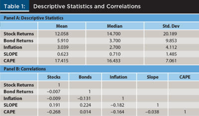
Table 1 provides descriptive statistics and correlations for the principle variables. The descriptive statistics for the Ibboston data are well known and yield few surprises. Stocks notably outperformed bonds, but were considerably more variable. The correlations of the variables did provide new insight, however. Notably, both the SLOPE and CAPE variables exhibited significant correlation with annual stock returns. Consistent with Kitces and Pfau (2015), with a correlation of –0.27, high CAPE values tended to be associated with low stock returns. With a correlation of 0.19, SLOPE exhibited a correlation with annual stock returns to almost as significant a degree, albeit in the opposite direction. And interestingly, SLOPE and CAPE were almost completely uncorrelated with each other, consistent with the notion that they likely capture different risks associated with equity returns.
For a baseline case, this study followed Bengen (1994) and constructed an estimate for each year in the dataset for which a 30-year retirement portfolio may be evaluated. The estimate consisted of the value path of a retirement portfolio that followed a given portfolio allocation and withdrawal rate. It assumed that the initial value of the portfolio was $100, that the retiree withdraws the given percentage of the portfolio in the first year of retirement, and in subsequent years withdraws that same dollar amount adjusted by the rate of inflation. A total of 59 overlapping 30-year periods comprised the dataset. For various possible withdrawal rates and portfolio allocations, Table 2 summarizes the performance of this retirement portfolio.
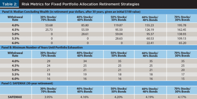
For each of the 59 overlapping 30-year periods, each withdrawal rate and portfolio allocation yielded a concluding portfolio value, expressed in retirement year dollars, and depended on the historical path of market variables. Panel A of Table 2 illustrates for each combination the median concluding portfolio value, given the $100 initial value. Consider one example: a portfolio consisting of 50 percent stocks and 50 percent bonds, in which the retiree withdraws 4.5 percent of the portfolio in the first year and adjusts this amount for inflation annually. For this example, the median concluding portfolio value of the 59 historical 30-year periods was $95.50. By contrast, if a withdrawal rate of 6 percent was established for the same portfolio allocation, the median portfolio was exhausted by the conclusion of 30 years, and was thus worth $0.
Panel A of Table 2 provides a rough indication of the rationale behind Bengen’s joint conclusion that retirees can reasonably expect their retirement assets to last for a 30-year retirement if they follow the 4 percent rule, and that they should maintain a 50 percent to 75 percent equity allocation. Relatively high withdrawal rates and relatively low equity exposure can combine to exhaust a retiree’s portfolio before the hypothetical 30-year retirement has concluded.
This pattern may be seen in Panel B of Table 2. For each of the 59 retirement years, the number of years the portfolio would survive was computed for each withdrawal rate/portfolio allocation pairing.2 Panel B illustrates, for each combination, the minimum number of years that the portfolio would last before it was exhausted, under the assumption that historical investment returns were realized. Naturally, as the withdrawal rate increases, this “worst-case” scenario gets worse—the minimum number of years the portfolio will survive declines. The minimum number of years is reflective of the volatility of the portfolio. The worst-case outcome tends to be worse with high-variability portfolios.
However, portfolio variability did not directly translate into retirement risk, as Table 2 illustrates. This is because the variability was augmented by compensation for the higher variability in the form of higher return. Because portfolios that are tilted more heavily toward stocks have significantly outperformed those tilted toward bonds, equity-heavy portfolios are to a retiree, in a sense, “less risky” than their bond-laden counterparts. To illustrate this, Panel C of Table 2 provides the SAFEMAX measure of Bengen (1994), which is the withdrawal rate that ensures, given the historical data, that a retirement portfolio will last at least 30 years. Increasing the percentage of stock holdings from 30 percent to 70 percent of the portfolio increased SAFEMAX from 3.95 percent to 4.17 percent, implying a “safe” income increase of about 5 percent.
The SLOPE Risk-Aversion Strategy
Presumably, financial planners will fix their client portfolios to a portfolio allocation and withdrawal rate that is a reflection of their risk tolerance, required rate of return to meet their goals, their constraints, and the practitioner’s capital market expectations. The tradeoffs of these choices are illustrated in Table 2.
Inverted yield curves are known to imperfectly forecast recessions in the United States; therefore, this study proposed a simple dynamic strategy that financial planners may impose on a retiree’s portfolio allocation in response to inverted yield curves. Specifically, if the yield curve is inverted (i.e., if SLOPE is less than zero) at the time of the annual evaluation, then reallocate the retiree’s portfolio defensively to an allocation of 20 percent stocks and 80 percent bonds. Otherwise, keep the portfolio weights balanced at their fixed allocations.
Results
Table 3 illustrates the results of employing the SLOPE risk-aversion strategy. Several implications are immediately apparent. Most notably, the strategy appears to dramatically increase the effectiveness of equity-heavy portfolio allocations. This was the case when withdrawal rates were relatively low. For example, when the withdrawal rate was 4 percent and the portfolio allocation was set at 70 percent stocks, the standard strategy illustrated in Table 2 implied that the median concluding wealth after 30 years was $195.78, and that the minimum time to portfolio exhaustion was 35 years. However, using the SLOPE risk-aversion strategy, the median concluding wealth was $242.41 (23.7 percent higher than the standard strategy) and the minimum years until portfolio exhaustion was 50, which was the maximum possible. Of course, keep in mind that these were historical returns. Asset returns in the United States may not be able to repeat the remarkable return profile they have exhibited over the last 90 years or so. Nonetheless, the results in Table 3 illustrate the potential benefits of reducing the economic risk that often accompanies an inverted yield curve.
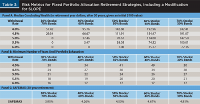
Incorporating the SLOPE as a defensive tool in this way reduces the lifetime risk of the retirement portfolio. Ironically, this risk reduction would not necessarily be picked up by the conditional standard deviation of stock price returns alone. Including only years when the yield curve was downward sloping, the standard deviation of the annual equity returns was 19.04 percent. When it was flat or upward sloping, that standard deviation was slightly higher, at 20.68 percent. Standard deviation, however, captured both positive and negative variation. By taking the downward-sloping yield curve as a defensive signal and shifting the allocation toward bonds, the hypothetical retiree was nonetheless able to limit downside risk. The reason lies in the means of the two yield curve slope states. When the yield curve was downward sloping, the (arithmetic) average annual stock market return was 9.12 percent. When it was upward sloping, it was 13.29 percent—a more than 400-basis point difference.
Further, this wasn’t just driven by outliers; the median returns exhibited a similar discrepancy: 11.35 percent to 16.25 percent. Indeed, the three worst annual returns: –43.3 percent in 1931; –35 percent in 1937 and; –37 percent in 2008 all took place in upward-sloping yield curve environments. Despite this, considerable underperformance was avoided by limiting exposure to equities when the yield curve sloped negatively. For example, when SLOPE was negative at the beginning of the year, the market returns for the year historically have been negative 43 percent more often than when SLOPE was positive.
Reducing the exposure to underperforming markets reduced client risk despite the similar standard deviations of equities.3 By reducing this exposure, it potentially allowed the client to take on a more variable portfolio allocation in non-inverted slope years.
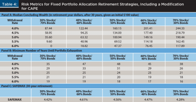
Kitces and Pfau (2015) undertook a similar kind of retiree portfolio modification when they proposed the use of the CAPE measure to dynamically adjust the portfolio allocation. Although they explored several methods by which the CAPE measure may be implemented, Table 4 demonstrates a simple version of that strategy—specifically, one in which the retiree had a fixed portfolio allocation and withdrawal rate. Then, that base strategy was modified such that if CAPE was “high,” the retiree held a defensive portfolio consisting of 20 percent stocks and 80 percent bonds. If CAPE was “low,” then the base strategy was modified aggressively such that the portfolio consisted of 80 percent stocks and 20 percent bonds. CAPE was considered “high” when it began the year by exceeding 4/3 of its median value to that point in time. CAPE was considered “low” when it began the year lower than 2/3 of its median value to that point in time.
Table 4 indicates the benefit of this kind of valuation rebalancing. Reaffirming Kitces and Pfau (2015), both the median concluding wealth at the end of the 30-year period, and minimum number of years until portfolio exhaustion were notably higher than the base case strategy. In all cases, median concluding wealth was higher than even under the SLOPE risk-aversion strategy. However, it is interesting to note that when the base portfolio allocation was rather aggressive, the minimum number of years until portfolio exhaustion was notably lower than the SLOPE strategy. While the CAPE modification was very effective at increasing expected concluding wealth, it did not imply a dramatic increase in the minimum number of years to portfolio exhaustion relative to the base case. It did not notably reduce the shortfall risk to the retiree. For aggressive portfolio allocation, however, the SLOPE strategy did.
This raises a natural question. Since both the CAPE and SLOPE strategies are so easy to implement—both only require an annual rebalance as implemented here—can they be used effectively together? Table 1 indicates a –0.038 correlation between CAPE and the slope of the yield curve. This is economically insignificant, and suggests that perhaps the benefits of each strategy are sufficiently dissimilar that they may be used effectively in conjunction with one another.
As a final strategy, consider the following: begin with the base case of a given portfolio allocation and selected withdrawal rate. If SLOPE is negative at the beginning of the year, assume a defensive strategy of 20 percent stocks and 80 percent bonds. Further, if CAPE is high, also assume this defensive allocation. If CAPE is low, take an aggressive strategy of 80 percent stocks and 20 percent bonds—unless SLOPE is negative, and then remain defensive. Call this the SLOPE-CAPE strategy. For clarity, Panel A of Table 5 summarizes the contingent positions held by the client under this strategy, while Panel B illustrates the historical relative frequency of the various states.
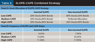
Table 6 provides a solid indication that this combination strategy can be very effective. It is an unambiguous improvement over the baseline strategy. It is an unambiguous improvement over the CAPE strategy also. In all cases, the minimum time to portfolio exhaustion was equal to or greater than the base CAPE strategy. The improvement, as would be expected given the performance of the SLOPE strategy demonstrated in Table 3, was particularly pronounced when the base portfolio allocation leaned more heavily toward equities. For example, consider a base portfolio allocated 70 percent stocks and 30 percent bonds, with a 4 percent withdrawal rate. The combination strategy yielded a median concluding portfolio wealth of $272.20, and in none of the historical simulations was the portfolio exhausted. By comparison, the CAPE strategy yielded a median concluding portfolio wealth of $244.33, and a minimum exhaustion time of 38 years.
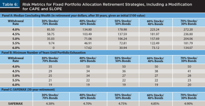
Perhaps the clearest example of the SLOPE-CAPE strategy is the increased “safe” withdrawal rate, at least given the historical returns with which we are working. The base case strategy due to Bengen (1994) allowed a maximum SAFEMAX of 4.20 percent, achieved with a 50 percent/50 percent portfolio allocation. The SLOPE-CAPE strategy yielded its highest SAFEMAX from a 70 percent/30 percent allocation, and this value was 4.90 percent. This is a nontrivial lifestyle improvement for the retiree. For a $1.25 million retirement portfolio, this 0.70 percent increase in the withdrawal rate implies an increase in annual income of more than $8,750. This is a roughly 16 percent income increase over the $52,500 that a 4.2 percent withdrawal rate would achieve. Again, this is a simple, once-a-year rebalance.
Implications for Financial Planners
The primary implication of this research is that the SLOPE risk-aversion strategy appears to allow the client to increase their equity allocation in non-inverted slope years, relative to the base-case Bengen (1994) strategy. Using historical returns, it appears this use of the SLOPE risk-aversion strategy allows a significant decrease in the shortfall risk of the retirement portfolio. Whether the goal of the client is to bequeath additional assets to heirs, or to enjoy an improved retirement lifestyle, the incorporation of this simple portfolio reallocation contingent upon the slope of the yield curve appears to significantly improve the client’s financial outlook in retirement.
Research has indicated that an inverted yield curve has forecasting power to predict recessions. Estrella and Mishkin (1998) provided one example, and Erdogan, Bennett, and Ozyildirim (2015) provided a more recent one. By using the yield curve to potentially bypass the added risk that accompanies recession, a retiree may be able to increase the safe withdrawal amount from their portfolio.
Kitces and Pfau (2015) found that dynamically modifying the portfolio to account for market valuation can improve the performance for retirees as well. This study confirmed that finding, and further found that a combination strategy that employs both the CAPE ratio and the SLOPE strategy was very effective and easy to implement. Both the slope of the yield curve and the CAPE ratio are readily available. For example, the Treasury data necessary to compute SLOPE can be found each morning in the Wall Street Journal, while the CAPE ratio may be readily found on many websites, such as www.multpl.com.
Further, the strategies outlined in this research that employ these variables are inexpensive to implement, as they require only annual rebalancing. The combined strategy employing both CAPE and SLOPE, particularly if a client chooses a relatively aggressive portfolio allocation, can increase SAFEMAX to 4.90 percent. This maximum safe withdrawal rate implies an improvement (using historical data) over that which is possible using the basic Bengen (1994) method (maximum of 4.20 percent), or the CAPE-inspired dynamic strategy (maximum of 4.61 percent).
A natural question for the financial planner, weighing his or her fiduciary responsibility, is: increasing the equity allocation in non-inverted SLOPE years can increase SAFEMAX, but what about the increased risk this implies? Is such a risk increase appropriate? The answer to this question is client specific. However, it is important to keep in mind that in many of the riskiest years, allocation strategies that depend on the slope of the yield curve will be highly defensive (20 percent equities, 80 percent bonds). Indeed, Table 5 indicates that historically SLOPE has been negative about 30 percent of the time, meaning that the defensive allocation would occur that frequently (and even a little more frequently if the CAPE-SLOPE strategy is pursued). Viewed in this light, it may be appropriate to think of the more aggressive stance in the non-inverted SLOPE years as compensating for the decreased equity allocation in the inverted years. With this tradeoff in mind, the financial planner can then appropriately advise the client of the risk profile of the SLOPE risk-aversion strategy.
Whether the recommendation is Bengen (1994), Blanchett (2007), or Kitces and Pfau (2015), it has long been asserted that a constant portfolio allocation, rebalanced annually, provides a simple and efficient method for the construction of a retirement portfolio. Although this research did not dispute that tradition, it suggested that a simple dynamic reallocation strategy that uses the slope of the yield curve may significantly improve the efficiency of the retirement portfolio.
Specifically, this research suggested that an inverted yield curve was indicative of potential risk to a retirement portfolio, and financial planners may want to regard an inverted yield curve during an annual rebalancing as an indicator to reduce client portfolio risk. By reducing equity exposure for clients at these times, a financial planner may be able to significantly mitigate a sizeable portion of retirement risk, allowing increased judicious risks to be taken at other times, resulting in a higher safe withdrawal rate for the client.
Endnotes
- Arbitrarily, this study used 10-year Treasury rates as the proxy for the “long” end of the yield curve, and three-month Treasury rates as the proxy for the “short” end of the yield curve. This selection was made primarily because of data availability. These two rates had such high correlations with other potential proxies for short- and long-term rates, respectively, that the particular choice of Treasury expirations was very unlikely to affect the results.
- To get a sense of the length of time the portfolio would last, the periods were extended to 50 years. To extend this for the latter part of the sample, this study followed Bengen (1994) and used the series’ averages to extend the hypothetical retirement period beyond the dataset as necessary.
- Unreported, the standard deviation of the concluding retiree wealth dropped significantly when the SLOPE risk-aversion strategy was employed.
References
Bengen, William P. 1994. “Determining Withdrawal Rates Using Historical Data.” Journal of Financial Planning 7 (4): 171–180.
Blanchett, David M. 2007. “Dynamic Allocation Strategies for Distribution Portfolios: Determining the Optimal Distribution Glide Path.” Journal of Financial Planning 20 (12): 68–81.
Blanchett, David M. 2015a. “Revisiting the Optimal Distribution Glide Path.” Journal of Financial Planning 28 (2): 52–61.
Blanchett, David M. 2015b. “Initial Conditions and Optimal Retirement Glide Paths.” Journal of Financial Planning 28 (9): 52–60.
Campbell, John Y. and Robert J. Shiller. 1998. “Valuation Ratios and the Long-Run Stock Market Outlook.” Journal of Portfolio Management 24 (2): 11–26.
Campbell, John Y. and Samuel B. Thompson. 2008. “Predicting Excess Stock Returns Out of Sample: Can Anything Beat the Historical Average?” Review of Financial Studies 21 (4): 1,509–1,531.
Delorme, Luke F., 2015. “Confirming the Value of Rising Equity Glide Paths: Evidence from a Utility Model.” Journal of Financial Planning 28 (5): 46–52.
Erdogan, Oral, Paul Bennett, and Cenktan Ozyildirim. 2015. “Recession Prediction Using Yield Curve and Stock Market Liquidity Deviation Measures.” Review of Finance 19: 407–422.
Estrella, Arturo and Frederic S. Mishkin. 1998. “Predicting U.S. Recessions: Financial Variables as Leading Indicators.” Review of Economic Statistics 80 (1): 45–61.
Homer, Sidney. 1963. A History of Interest Rates. New Brunswick, N.J.: Rutgers University Press.
Kitces, Michael E. and Wade D. Pfau. 2015. “Retirement Risk, Rising Equity Glide Paths, and Valuation-Based Asset Allocation.” Journal of Financial Planning 28 (3): 38–48.
Pfau, Wade D. 2012. “Capital Market Expectations, Asset Allocation, and Safe Withdrawal Rates.” Journal of Financial Planning 25 (1): 36–43.
Pfau, Wade D., and Michael E. Kitces. 2014. “Reducing Retirement Risk with a Rising Equity Glide Path.” Journal of Financial Planning 27 (1): 38–45.
Shiller, Robert J. 1990. Market Volatility. Cambridge, Mass.: The MIT Press.
Citation
Fink, Jason D., and Kristin E. Fink. 2016. “A Dynamic Yield Curve-Based Approach to Retiree Portfolio Allocation.” Journal of Financial Planning 29 (9): 50–57.