Journal of Financial Planning: October 2015
Wade D. Pfau, Ph.D., CFA, is a professor of retirement income at The American College and a principal at McLean Asset Management. He is a two-time recipient of the Journal’s Montgomery-Warschauer Award. He hosts the Retirement Researcher website, RetirementResearcher.com.
Executive Summary
- Variable spending strategies can be situated on a continuum between two extremes: spending a constant amount from the portfolio each year without regard for the remaining portfolio balance, and spending a fixed percentage of the remaining portfolio balance.
- Variable spending strategies seek a compromise between these extremes by avoiding too many spending cuts while also protecting against the risk that spending must subsequently fall to uncomfortably low levels.
- This paper reviews two basic categories for variable spending rules: decision rule methods and actuarial methods.
- Ten strategies were compared using a consistent set of portfolio return and fee assumptions using the following XYZ formula to calibrate initial spending: the client willingly accepts an X percent probability that spending falls below a threshold of $Y (in inflation-adjusted terms) by year Z of retirement.
- This paper provides 13 numbers to summarize the performance of a strategy, including the initial spending rate, the evolution of real spending over 30 years at different points in the distribution of outcomes, and the distribution of remaining real wealth after 30 years.
Bengen (1994) introduced the concept of the 4 percent rule for retirement withdrawals. He defined the sustainable spending rate as the percentage of retirement date assets that can be withdrawn, with this amount adjusted for inflation in subsequent years, such that the retirement portfolio is not depleted for at least 30 years. Specifically, Bengen found that a 4 percent initial spending rate would have been sustainable in the worst-case scenario from U.S. historical data over rolling 30-year periods with a stock allocation of between 50 percent and 75 percent.
In an attempt to illustrate the importance of the sequence of investment returns on retirement spending outcomes, which highlighted how it is wrong to base a sustainable spending rate on a fixed average return assumption plugged into a spreadsheet, Bengen (1994) used a number of simplifying assumptions. Among these was the previously mentioned constant inflation-adjusted spending assumption. This was a simplification to obtain a general guideline about feasible retirement spending.
Although the assumption may reflect the preferences of many retirees to smooth their spending as much as possible, typical clients can be expected to vary their spending over time. Clients will generally not keep their spending constant as their portfolios plummet toward zero. And constant spending from a volatile portfolio is a unique source of sequence of returns risk that can be partially alleviated by reducing spending when a portfolio drops in value.
But how exactly should clients adjust their spending patterns in response to changes in the value of their retirement portfolios? Countless variations on spending rules are discussed in outlets ranging from research papers to internet discussion boards. The purpose of this paper is to identify and classify key variable spending strategies, and to develop simple metrics to evaluate and compare the strategies on an equal basis.
Forget the “Failure Rate”
As will be discussed, the frequently used “failure rate” metric should not be applied to variable spending rules. Other approaches are needed. The aim here is to assist financial planners and their clients in figuring out which sort of variable spending strategy will be most appropriate for their situations. This holistic evaluation is important for a number of reasons.
To begin with, variable spending rules are usually described and evaluated using different data and assumptions. As such, if one rule suggests a 6 percent withdrawal rate while another suggests a 3 percent withdrawal rate, it is difficult to know whether the first rule is really twice as powerful. The difference could just reflect different underlying assumptions, such as higher market returns. It is important to use the same set of capital market and fee assumptions to properly compare strategies.
Financial planners must also worry about where clients are situated in the distribution of possible spending and wealth outcomes. Many trade-offs are involved with building a retirement income strategy, and one metric cannot summarize the overall performance of a strategy. Spending more at the start of retirement creates a greater risk for having to spend less later. A more aggressive asset allocation creates greater upside potential for spending growth and legacy, but it leads to greater downside risk as well. Naturally, regarding legacy, greater spending implies that fewer assets will remain. Spending can evolve differently depending on the random sequence of market returns. Clients must decide where to focus their concerns.
The traditional failure rate measure often employed by safe withdrawal rate studies (those that calculate the probability of portfolio depletion) cannot be used to compare variable spending strategies. This approach only tracks portfolio depletion, and different variable strategies may imply different spending levels just prior to wealth depletion. For instance, a 6 percent variable spending strategy may cause spending to fall to $20,000 per year in the period leading up to portfolio depletion, while a 3 percent strategy might result in spending at $50,000 until depletion. Failure rates ignore this important distinction because the depletion event is all that matters. This is important because it reflects a general theme in the variable withdrawal rate literature: the more the client is willing to let their spending drop in retirement, the higher the initial spending rate they may use.
A related problem is that some variable spending strategies can technically never fail. For instance, when calculating spending as a percentage of remaining assets, even a 99 percent withdrawal rate never runs out. Portfolio failure rates also do not reflect a client’s entire household balance sheet of assets for income generation. Cutting spending from a portfolio may not be so disastrous for clients who receive plenty of income from other sources such as Social Security, pensions, and income annuities. It is important to consider how potential spending reductions from a portfolio will impact the overall lifestyle of the client after also incorporating all of their other non-portfolio sources of income. Failure, defined strictly as investment portfolio depletion, is not the whole story.
The failure rate is also an extreme outcome measure that puts weight only on financial wealth depletion. Client spending potential is irrelevant. Clients must find an appropriate personal balance between the aims of spending more and then having to make potentially larger subsequent cutbacks in the event of a long life and a sequence of poor market returns. By focusing only on the failure rate, clients may end up bequeathing a large amount of assets and not enjoying their retirements as much as possible.
An Alternative to Failure Rates
As an alternative to failure rates, this paper suggests comparing the distribution of outcomes for spending and remaining wealth for different strategies, and calibrating initial spending rates using the following customized “XYZ formula” determined by the financial planner and client:
XYZ Formula = Client willingly accepts an X percent probability that spending falls below a threshold of $Y (in inflation-adjusted terms) by year Z of retirement.
For instance, instead of accepting a 10 percent chance of failure within the first 30 years of retirement, an XYZ rule could be that the client accepts a 10 percent chance that their spending level falls below an inflation-adjusted $60,000 by the 30th year of retirement. This calculation can incorporate Social Security and other income sources as well, and it provides a way to compare strategies while otherwise dealing with the reality that higher initial spending rates can be justified if spending is subsequently allowed to drop more steeply.
The formula provides a controlled anchor for those spending drops. When combined with consistent market assumptions and a view of the entire distribution of outcomes, financial planners can compare different variable strategies on an equal footing.
Decision Rules vs. Actuarial Methods
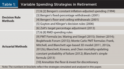
This review provides a summary of research on variable spending by identifying and describing key representative variable spending strategies and classifying them into a general taxonomy with two subsets: decision rule methods and actuarial methods.1 Key examples of each are shown in Table 1.
Though there are exceptions, it is possible to generalize a few important distinctions from these methods. Among these distinctions, decision rule methods frequently share elements of the probability-based school of thought, while advocates of actuarial methods often identify more with the safety-first school (See Pfau and Cooper (2014) for more on these schools of thought).
For instance, decision rule methods demonstrate more willingness to start spending at a higher level than justified by the bond yield curve, with an expectation that future portfolio growth from stocks can be counted upon to justify a higher spending rate currently. Meanwhile, with actuarial methods, spending may start at a lower level. Spending will only increase in the event that upside potential has been realized. There is a greater recognition of the notion that stock investments are still risky even after long holding periods, so efforts to “amortize the upside” through higher spending may backfire on the client.
Related to this, decision rules generally try to keep spending at a steadier level and only make spending adjustments when deemed essential. Actuarial methods may call for more frequent spending adjustments. Actuarial advocates often suggest that those seeking smoother spending should use a less volatile portfolio. For actuarial methods, spending volatility is more directly linked to investment volatility, and it is the asset allocation lever that should be used to reduce spending volatility rather than any other sort of smoothing technique. Any effort to keep spending constant from a volatile portfolio creates greater risk for even greater subsequent spending declines.
Beyond these differing views of market risk, decision rule methods generally adopt a conservative planning horizon beyond life expectancy (such as 30 or 40 years), while actuarial methods make decisions based on a dynamically adjusting time horizon linked to the remaining life expectancy as retirement progresses.
Finally, those using decision rule methods will generally be more comfortable in formulating their spending parameters using historical market data, whereas actuarial method advocates will be more willing to incorporate updated market return expectations as the spending plan is restructured regularly throughout retirement.
Testing Decision Rule Methods
The first method to be tested, so that it may serve as a baseline for comparison, is the [1] original constant inflation-adjusted withdrawal strategy introduced by Bengen (1994). This basic spending rule involves adjusting spending annually for inflation and maintaining constant inflation-adjusted spending for as long as possible until the portfolio depletes.
A test of a variant in which [2] the annual spending adjustments equal inflation less 1 percentage point was also tested. This allows for a higher initial spending rate, followed by subsequent real spending declines. This variant may appeal to those who do expect their spending to naturally decline with age, as it provides a mechanical way to front load spending. More generally, any client-specified targeted spending path could be simulated in this way.
The next decision rule is the opposite of constant inflation-adjusted spending. Bengen (2001) described it as [3] fixed-percentage withdrawals. This rule calls for users to spend a constant percentage of the remaining portfolio balance in each year of retirement. This rule never depletes the portfolio.
Cotton (2013) formalized how there is no sequence of returns risk with a constant percentage strategy. Intuitively, the lack of sequence risk can be understood as the fact that this strategy provides a clear mechanism for reducing spending after a portfolio decline. As with investing a lump sum of assets, the specific order of returns makes no difference to the final outcomes realized with this strategy. As such, financial planners can expect the sustainable spending rate to be higher than with constant inflation-adjusted withdrawals. As for disadvantages, spending can become extremely volatile with this strategy, particularly if combined with volatile investments. This means that it can be difficult for clients to budget in advance.
The fixed percentage and the constant (inflation-adjusted) rules represent the two extremes on a spectrum of possible choices. With Bengen’s (2001) fixed percentage rule, spending can be very volatile, but the portfolio technically cannot be depleted. Meanwhile, a constant amount does keep spending more predictable as long as assets remain, but the portfolio can be depleted and spending can fall to zero. Neither extreme will be ideal for most clients. The other decision rule methodologies seek to provide a compromise of sorts between these two extremes by having a mechanism to smooth spending adjustments made in response to market volatility.
Bengen (2001) described [4] floor-and-ceiling withdrawals as one such spending compromise. This method begins by applying the fixed percentage rule, which allows greater spending when markets do well and forces spending reductions when markets do poorly. Bengen added hard dollar ceilings and floors on spending. Spending would not be allowed to rise above the ceiling set at 20 percent higher than the real value of the first year’s withdrawal, whereas spending would not be allowed to fall by more than 15 percent below the real value of the first year’s withdrawal. This keeps spending from drifting too far from its initial levels as a way to smooth spending fluctuations. It is important to recognize that the hard dollar floor on spending imposed by this rule restores the possibility for portfolio depletion. The failure rate comparison would be less meaningful for this rule if spending was already lower in the period before wealth depletion than with constant inflation-adjusted spending. A willingness to cut spending when markets do poorly does justify a higher initial spending rate. Bengen determined that this floor-and-ceiling rule increased the historical worst-case initial spending rate by 10 percent.
The next decision approach is known as the [5] Guyton and Klinger spending decision rules, which is a derivation from work by Guyton (2004) and Guyton and Klinger (2006). The basic components of these spending rules include a spending adjustment for inflation unless the portfolio has a negative return in the previous year and this year’s withdrawal rate (current spending divided by remaining assets) is higher than the initial withdrawal rate at the retirement date.
Additionally, the “prosperity rule” increases spending by 10 percent in any year that the current withdrawal rate falls to 20 percent less than its initial level. The “capital preservation rule” cuts spending by 10 percent during the first 15 years of retirement if the current withdrawal rate rises to be 20 percent more than its initial level. With these decision rules, spending can increase faster than inflation when the markets are doing well and fall even in nominal terms when the portfolio is losing value.
A final example in the decision rules category is the [6] target percentage adjustment method introduced by Zolt (2013). This method is a hybrid between decision rules and actuarial methods, though it is classified here as a decision rule method because of the simple spending rule that defines whether spending adjusts for inflation. Given a fixed-return assumption and a 45-year time horizon, Zolt calculated a critical path for how much wealth should remain in each year of retirement. In any year that remaining wealth is higher than the critical number from his calculation, spending adjusts for inflation. However, in any year that wealth falls below where it should be as implied by this critical path, no inflation adjustment is made. Throughout retirement, sometimes spending adjusts for inflation and sometimes it stays fixed. Zolt considered other variants for how much to adjust spending depending on the relationship between wealth and the critical path calculations. This study simulates the version by including a 45-year planning horizon, 3 percent inflation, and an 8.6 percent portfolio return.
Testing Actuarial Methods
Actuarial methods generally have clients recalculate their sustainable spending annually based on the remaining portfolio balance, remaining longevity, and expected portfolio returns. These methods can generally be represented with the Excel PMT function:
PMT (rate, nper, pv, fv, type)
Given an expected return for investments (rate), the planning horizon (nper), the current size of the financial portfolio (pv), the desired amount of remaining wealth at the end of the planning horizon (fv), and a value of 1 for type if withdrawals are made at the start of the period, this formula provides the sustainable spending amount. If the rate is expressed in inflation-adjusted terms, the answer would imply a stronger opportunity to enjoy continued inflation-adjusted spending from this level. Additionally, fv could be a value greater than zero if the client seeks to leave a bequest or to preserve a portion of the portfolio for other purposes.
This calculation could be repeated annually, reflecting changes in rate, nper, and pv, which would then provide clients with a sustainable spending amount for each year. Remaining portfolio assets will clearly change over time, and circumstances may also call for a change in expected market returns. A dynamic measure of remaining life expectancy is also important, as withdrawal rates can increase when the remaining time horizon shortens.
Steiner (2014) suggested that users may smooth spending adjustments relative to the changes implied by this formula. Not all would agree, as Waring and Siegel (2015) noted that a less volatile asset allocation is a safer way to smooth spending fluctuations. The PMT formula does make clear that market volatility is the main source for spending fluctuations. Waring and Siegel argued that clients who seek stable spending should create a less volatile portfolio to be logically consistent with their choices.
A basic form for the actuarial method is to use the Internal Revenue Services’ required minimum distribution (RMD) model as a more general guide for sustainable spending. In an effort to get those benefiting from tax deferral to eventually pay taxes, the RMD rules indicate a by-age percentage that must be withdrawn from tax-deferred accounts.
Blanchett, Kowara, and Chen (2012) and Sun and Webb (2012) both studied the RMD rule as a spending option and found it to be a reasonable strategy that roughly approximates more sophisticated attempts to optimize spending. The RMD rule contains the actuarial components of spending a percentage of remaining assets calibrated to an updating remaining life expectancy, covering the nper and pv aspects of the PMT formula. An RMD deficiency is that it does not provide a mechanism for users to adjust the value of rate beyond whatever government policymakers initially assumed when developing their RMD framework. This paper simulates the [7] straightforward RMD rule, which does not have flexibility to calibrate to an XYZ rule, as well as a [8] modified version of the RMD rule in which the RMD spending rates are adjusted to comply with the parameters of the XYZ rule.
The next simulated method is to use the [9] PMT formula. Most recently, Waring and Siegel (2015) called this the “annually recalculated virtual annuity” (ARVA) approach. Steiner (2014) called this method the “actuarial approach.” Users at the Bogleheads Forum (2015) collectively developed a variant of this approach that they named “variable percentage withdrawal.” The approach recognizes that the amount someone can spend in each year of retirement can be determined through a simple annuity calculation for a spending rate assuming a fixed portfolio return and remaining time horizon. This calculation can be updated annually for the new portfolio balance, any changes to the expected return, and an adjustment for remaining longevity. The method does not provide a clear baseline about assumptions for which all users would agree. To show how the method may work in practice, this paper simulates a variant using modeled 10-year Treasury rates for the expected returns and rounded life expectancy numbers used in the RMD rule. This is the only other method that is not calibrated to the XYZ formula.
A number of other more sophisticated actuarial methods also incorporate Monte Carlo simulations to calibrate spending based on a specified probability of success or failure. Though these will not be simulated here, they are worth mentioning, as they provide more sophisticated versions of the PMT formula. Examples include the age-based, three-dimensional distribution model developed by Frank, Mitchell, and Blanchett (2011, 2012a, 2012b), the mortality-updating constant probability of failure withdrawal method of Blanchett et al. (2012), and the simple formula for retirement withdrawals introduced by Blanchett (2013). The latter allows users to input their preferred asset allocation, expected portfolio returns, level of portfolio fees, remaining life expectancy, and targeted probability of success in order to obtain a customized withdrawal rate. Though these methods are more sophisticated, the underlying PMT formula remains as the philosophical core of the spending recommendations.
A final method simulated here is to partially annuitize with an inflation-adjusted income annuity to cover essential spending needs, and to then spend more aggressively from remaining assets. The assumed annuity payout rate is 3.75 percent, which matches the inflation-adjusted option available to a 65-year-old couple with joint and 100 percent survivor’s income in early 2015. With the XYZ formula, the client annuitizes enough to cover their minimum $Y floor. The remainder of spending will be determined with a more aggressive version of the Guyton and Klinger (2006) decision rules.
Methodology
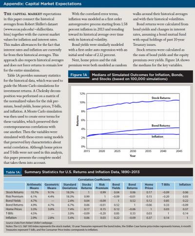
Each strategy was simulated using 10,000 Monte Carlo simulations for stock and bond returns. The details of the underlying market simulations are provided in the appendix. These simulations reflect the lower bond yields available to retirees today, but they do include a mechanism for interest rates to gradually increase over time, on average. Bond returns were calculated from the simulated interest rates and their changes. Stock returns were calculated by adding a simulated equity premium on top of the simulated interest rates.
All strategies were simulated with the same asset allocations and portfolio returns in order to make the results comparable. Strategies were simulated with annual data, assuming withdrawals were made at the start of each year, using annual rebalancing to restore the targeted asset allocation, and deducting a 0.5 percent fee from remaining portfolio assets at the end of the year. The tax implications for different spending strategies were not otherwise considered.
For each strategy, the initial spending rate is shown, with the assumption that retirement wealth is equal to $100,000 (see Table 2). Results are scalable for other wealth amounts. The distribution for spending amounts is shown for 10, 20, and 30 years into retirement. Additionally, the distribution of remaining wealth is shown after the 30th year of retirement. A consideration of spending and wealth are both important, as retirees should not be narrowly focused on a singular goal to avoid financial wealth depletion.
Financial goals for retirement can essentially be reduced to two competing objectives: (1) to support as much spending as feasible; and (2) to maintain a reserve of financial assets to support risk management objectives, such as protecting a household from expensive health shocks, divorce, unexpected needs of other family members, and severe economic downturns, or to otherwise provide a legacy.
In presenting outcomes, the part of the distribution of outcomes that should be highlighted is not completely clear, though retirees will surely wish to consider the implications for when markets do well and when markets do poorly. To demonstrate the range of possibilities, outcomes for spending and remaining wealth are shown for the 90th percentile (markets do well), 50th percentile (the mid-range outcome in which half can expect to do better and half worse), and the 10th percentile (markets do poorly).
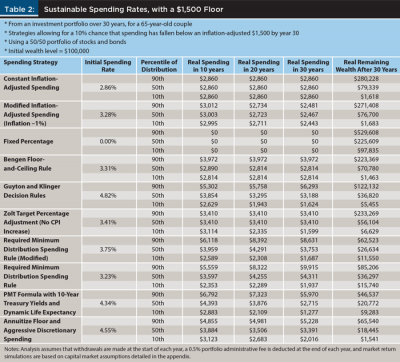
Table 2 presents outcomes for 10 different spending strategies, eight of which are calibrated using the XYZ rule. Again, this rule is defined as a client allowing for an X percent chance that spending will fall below $Y by year Z of retirement. The two strategies not calibrated are the RMD rule and the ARVA rule, as those strategies are strict about how retirement spending should be defined.
Results for Decision Rule Methods
Table 2 presents results for each strategy assuming an asset allocation of 50 percent stocks and 50 percent bonds. The XYZ formula applied in this table is that clients accept a 10 percent chance that spending falls below $1,500 (in inflation-adjusted terms) by year 30 of retirement. This constraint guides initial spending for eight of the 10 strategies. The rule does not otherwise build in a legacy objective, so all wealth is available for spending, and any legacy is unintentional and undesirable from a spending perspective.
The first strategy is constant inflation-adjusted spending, which Bengen (1994) popularized as the 4 percent rule. After incorporating 0.5 percent administrative fees and the lower interest rates available to clients at the present, the maximum sustainable initial spending rate that meets the requirements of the XYZ rule is 2.86 percent. For the $100,000 initial portfolio, this supports $2,860 in real spending across the entire distribution of Monte Carlo simulations for as long as wealth remains. At the 10th percentile, after 30 years of retirement, wealth is on the cusp of running out. With $1,618 remaining, the portfolio will be depleted in the 31st year. In the median outcome, almost 80 percent of the initial wealth remains after 30 years even after adjusting for inflation. Wealth grows by almost 2.8 times in real terms at the 90th percentile. This strategy does not take advantage of the upside potential from the investment portfolio. On the downside, spending is still maintained at a higher level up until the point of wealth depletion. Wealth does not fall to the $1,500 allowed threshold until wealth is gone, and then a large discrete drop in spending takes place.
The next strategy is similar to the constant spending rule, except that spending will grow at a rate less than the consumer price index (CPI). This provides a mechanical way to increase initial spending, with a built-in adjustment factor that will automatically reduce real spending over time. More generally, any predetermined spending pattern could be tested in a similar way. This rule also does not adjust spending to portfolio performance. The initial spending rate increases by 15 percent to 3.28 percent, at which point real spending will gradually decline subsequently. Real spending varies slightly across the distribution of outcomes to reflect the differing compounded inflation rates for the different Monte Carlo simulations. As for remaining wealth after 30 years, wealth may still be high except for the worst-case scenarios because the rule does not provide any upward adjustment for good market returns.
The third strategy is to spend a fixed percentage of the remaining portfolio balance. This rule could not be calibrated to the specified XYZ formula, so a spending rate of 0 percent was used. This is an exception. A later example will be used in which the formula will apply. The problem here is that there is no balance point for the XYZ formula. Higher spending rates cause spending to fall below the $1,500 floor too frequently. Additionally, lower spending rates cannot get spending above this floor often enough. With no withdrawals, the 30-year remaining wealth numbers indicate the growth of wealth across the distribution for the $100,000 available at the retirement date.
The next strategy is Bengen’s (2001) floor-and-ceiling rule. This rule shows the synergies that can develop when allowing spending to fluctuate with market returns. The initial spending rate can be increased to 3.31 percent, which is 16 percent more than a constant inflation-adjusted spending approach. Nevertheless, the hard spending floor supports spending at a level close to the same as before in the unlucky part of the distribution. Further, there is potential for further upside spending. After 30 years, the XYZ rule calibrated this strategy to be at the precipice of wealth depletion for the 10th percentile in year 30. At other points in the distribution, this strategy is a little more efficient in spending down wealth. With good market outcomes, wealth can still more than double, as the ceiling is not otherwise as high as it could have been when legacy is not an objective.
Next, the Guyton and Klinger (2006) decision rules allow initial spending to increase by 69 percent to 4.82 percent, relative to the Bengen (1994) baseline. The strategy provides greater upside spending potential and median spending remains higher as well. Although still calibrated to the XYZ formula, the 10th percentile spending is less than with constant inflation-adjusted spending. The strategy provides greater upside potential with some additional downside risk, although the minimum floor identified by the client is still being protected as well as with other spending rules. The strategy is more efficient in spending down wealth, as lower wealth balances remain after 30 years, ensuring that retirees could enjoy much more of their potential spending throughout retirement.
Zolt’s (2013) target percentage adjustment strategy was analyzed next. This approach allows for a 19 percent initial spending increase relative to constant inflation-adjusted spending. This strategy also uses wealth more efficiently than the baseline, although there is not a mechanism for spending to increase beyond the initial level when markets are doing well. It should be clear that such increases could be built in if desired by modifying the spending rule.
Results for Actuarial Methods
The actuarial methods were found to spend down wealth more efficiently. The first method evaluated was a modified version of the RMD spending rule. The modification was to scale up the spending rate above the RMD rule in order to calibrate the XYZ formula to retirement spending. The modified rule allows for an initial spending rate of 3.75 percent. With it, the distribution of spending widens, as an increasing percentage of the remaining portfolio is spent each year. At the median and 90th percentile, real spending grows at 10 and 20 years into retirement and then declines by year 30 as the spending rate becomes increasingly aggressive at higher ages. Real spending continuously declines at the 10th percentile to just above the $1,500 XYZ threshold at year 30. Wealth after 30 years is less across the distribution, implying that this strategy more efficiently spends down wealth.
The next strategy is the traditional RMD rule, which calls for a 3.23 percent withdrawal rate at age 65, a 3.65 percent withdrawal rate at 70, and so on. The straightforward RMD rule is not calibrated to the XYZ formula; it is more conservative. At the median and 90th percentiles, spending can be expected to continue growing in real terms throughout retirement. It declines at the 10th percentile, though it is still $1,937 after 30 years, which is above the XYZ threshold applied in other cases.
Testing of the PMT formula was performed next. This rule can be designed many different ways. The version shown implies aggressiveness as (1) remaining life expectancy is used for each year of retirement; and (2) as the nominal, rather than real, 10-year Treasury yield is used each year to calibrate spending. This suggests that the rule will start with higher spending, but that spending will decline throughout retirement, unless upside is realized through the 50/50 portfolio with a higher “expected” return than provided by Treasury yields. Spending could have been more aggressive if such a higher return from an investment portfolio was used in place of the Treasury rate, although this would increase downside risks as well. The initial spending rate is 4.34 percent, and at the median, spending holds relatively constant in real terms through the first 10 years of retirement.
The final method involved annuitizing the spending floor with an inflation-adjusted single premium immediate annuity (SPIA). Using 40 percent of assets, a 65-year-old couple annuitizing can obtain $1,500 of real income with a 3.75 percent payout rate for a joint and 100 percent survivor’s SPIA, which adjusts for CPI. The remaining 60 percent of the retirement portfolio can then spend down using the Guyton and Klinger (2006) decision rules. With these decision rules, spending can be more aggressive than shown earlier in the results table, because the XYZ formula for remaining assets allows for a floor of $0. Spending can start higher at 4.55 percent because it is allowed to fall more aggressively when market outcomes are poor, as the income annuity protects the client’s specified spending floor.
To better understand how the floor in the XYZ formula matters, Table 3 repeats the analysis by applying the XYZ formula with a floor level of $250 instead of $1,500. This allows for a higher initial withdrawal rate because spending is allowed to fall more steeply during retirement. Why might a client be willing to allow for greater declines? Aside from having greater flexibility to reduce spending, this may be an appropriate decision when a client’s risk capacity is greater because more income is available from outside the investment portfolio. A client who is able to cover their basic spending with Social Security and other pensions can view their portfolio withdrawals as being more discretionary in nature.
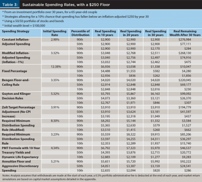
Modifying the XYZ formula to include a lower floor causes initial spending rates to increase notably for the Guyton and Klinger (2006) decision rules, Zolt’s (2013) target percentage adjustment, the modified RMD rule, and the floor annuitization strategy. The fixed percentage rule is also able to be calibrated with the lower floor, allowing for a 12.4 percent withdrawal rate. Because the floor is so low in Table 3, this high withdrawal rate is a manifestation of the idea that failure is not possible with a fixed percentage rule. For other spending rules, initial withdrawal rates do not change much, either because the XYZ formula was not applied or because the mechanical nature of spending changes do not provide a way for spending to be lowered enough in the lead up to depletion. Small differences can be found when the spending rate is a little higher because less wealth is needed at the end of year 30 to support the spending floor in the subsequent year.
Conclusions
A natural guideline for the retirement spending decision is to determine with the client what spending rate would satisfy their lifestyle goals. Beyond this, it is important to consider the client’s degree of spending flexibility to make cuts if necessary, as well as the client’s desire to maintain legacy wealth. Armed with this information, it is possible to consider the broad range of variable spending strategies and choose one that looks to best match the client’s goals. That is where this research’s framework can help with the decision-making process.
How should a client choose a spending method and parameterize the initial spending rate? This paper provides a framework to think about the important issues, such as spending flexibility, feelings about upside spending growth versus downside spending risks, the minimum spending threshold to be protected, desired direction of spending (for instance, whether to decrease spending over time), the appropriate planning horizon, and any legacy goals. With decisions made about these issues, clients can decide on an appropriate XYZ formula, and then compare the distributions of spending and wealth created by variable spending rules. Financial planners can use this toolbox of spending strategies to determine the most appropriate fit for different client circumstances.
As a general distinction, decision rule strategies tend to put retirement income spending rules in place at the start of retirement, while actuarial methods allow for more revision over time for the expected portfolio returns and remaining time horizon. In practice, however, financial planners will wish to return to the spending rules as a part of their client reviews to determine if further changes are warranted beyond the natural spending adjustments provided by the rules, or as client circumstances and spending needs change. All of the rules offer financial planners plenty of opportunity to continue engaging with their clients.
Endnote
- A third category of variable spending strategies is based on dynamic programming computational methods. These methods integrate spending and asset allocation decisions more completely and offer the most sophisticated models, but these methods are beyond the scope of this paper. Due to their mathematical complexity, they have not yet become a practical part of the toolkit for financial planners. For more information on dynamic programming methods, see Irlam (2014) or Irlam and Tomlinson (2014).
References
Bengen, William P. 1994. “Determining Withdrawal Rates Using Historical Data.” Journal of Financial Planning 17 (3): 172–180.
Bengen, William P. 2001. “Conserving Client Portfolios during Retirement, Part IV.” Journal of Financial Planning 14 (5): 110–119.
Blanchett, David M. 2013. “Simple Formulas to Implement Complex Withdrawal Strategies.” Journal of Financial Planning 26 (9): 40–48.
Blanchett, David, Maciej Kowara, and Peng Chen. 2012. “Optimal Withdrawal Strategy for Retirement-Income Portfolios.” Retirement Management Journal 2 (3): 7–20.
Bogleheads Forum. 2015. “Variable Percentage Withdrawal.” www.bogleheads.org/wiki/Variable_percentage_withdrawal.
Cotton, Dirk. 2013. “Clarifying Sequence of Returns Risk (Part 2, with Pictures!).” Retirement Café blog (September 20). theretirementcafe.blogspot.com/2013/09/clarifying-sequence-of-returns-risk_20.html.
Frank, Larry R., John B. Mitchell, and David M. Blanchett. 2011. “Probability-of-Failure-Based Decision Rules to Manage Sequence Risk in Retirement.” Journal of Financial Planning 24 (11): 44–53.
Frank, Larry R., John B. Mitchell, and David M. Blanchett. 2012a. “An Age-Based, Three-Dimensional Distribution Model Incorporating Sequence and Longevity Risks.” Journal of Financial Planning 25 (3): 52–60.
Frank, Larry R., John B. Mitchell, and David M. Blanchett. 2012b. “Transition through Old Age in a Dynamic Retirement Distribution Model.” Journal of Financial Planning 25 (12): 42–50.
Guyton, Jonathan T. 2004. “Decision Rules and Portfolio Management for Retirees: Is the ‘Safe’ Initial Withdrawal Rate Too Safe?” Journal of Financial Planning 17 (10): 54–62.
Guyton, Jonathan T., and William J. Klinger. 2006. “Decision Rules and Maximum Initial Withdrawal Rates.” Journal of Financial Planning 19 (3): 49–57.
Irlam, Gordon. 2014. “Portfolio Size Matters.” Journal of Personal Finance 13 (2): 9–16.
Irlam, Gordon, and Joseph Tomlinson. 2014. “Retirement Income Research: What Can We Learn from Economics?” Journal of Retirement 1 (4): 118–128.
Pfau, Wade D., and Jeremy Cooper. 2014. “The Yin and Yang of Retirement Income Philosophies.” SSRN working paper #2548114. ssrn.com.
Steiner, Ken. 2014. “A Better Systematic Withdrawal Strategy—The Actuarial Approach.” Journal of Personal Finance 13 (2): 51–56.
Sun, Wei, and Anthony Webb. 2012. “Should Households Base Asset Decumulation Strategies on Required Minimum Distribution Tables?” Center for Retirement Research at Boston College working paper 2012-10. crr.bc.edu.
Waring, M. Barton, and Laurence B. Siegel. 2015. “The Only Spending Rule Paper You Will Ever Need.” Financial Analysts Journal 71 (1): 91–107.
Zolt, David. 2013. “Achieving a Higher Safe Withdrawal Rate with the Target Percentage Adjustment.” Journal of Financial Planning 26 (1): 51–59.
Citation
Pfau, Wade D. 2015. “Making Sense Out of Variable Spending Strategies for
Retirees.” Journal of Financial Planning 28 (10): 42–51.