Journal of Financial Planning: October 2015
David D. Cho, Ph.D., is an associate professor of finance at Nova Southeastern University. His current research interests are in the areas of investments, credit markets, and financial econometrics.
Emre Kuvvet, Ph.D., is an assistant professor of finance at Nova Southeastern University. His research includes issues in market microstructure, corporate fraud, and political economy.
Executive Summary
- Despite lump-sum investing’s superior performance, dollar-cost averaging continues to be popular among investors.
- Much of the previous literature has used behavioral reasoning, seasonality, conditional expected returns, and mean reversion in stock prices to explain this popularity.
- Using a standard mean-variance analysis, this paper finds that dollar-cost averaging can be used to lower risk.
- Results suggest that depending on an investor’s level of risk aversion, dollar-cost averaging can be an optimal investment strategy.
Instead of investing money in one lump-sum, dollar-cost averaging (DCA) is a strategy where an investor invests money into risky assets by allocating equal dollar amounts over a period of time. Practitioners have championed this investment method for a long time, arguing that DCA minimizes losses in a portfolio’s value if the price of a risky asset gradually declines. Lump-sum investing is thus considered risky, as the price of a risky asset can immediately decline after investing. Proponents of DCA also claim that it can provide a lower average purchase price for a risky asset, suggesting that purchases of more risky assets with DCA when prices are declining will provide better returns than lump-sum investing.
Despite the fact that the majority of academic research has shown that DCA is inferior to lump-sum investing (as well as other investment strategies), the popularity of DCA remains high among practitioners and the investing public.
Previous studies have sought to explain the popularity of DCA via behavioral finance. Statman (1995) attributed the use of DCA to investor irrationality, proposing four behavioral explanations for the popularity of DCA: (1) prospect theory, which posits that people tend to give less weight to outcomes that are merely probable than to outcomes that can be obtained with certainty; (2) aversion to responsibility and regret; (3) cognitive errors caused by recent stock trends; and (4) a lack of self-control.
Leggio and Lien (2001) empirically tested Statman’s behavioral rationale for the persistence of DCA. However, their findings contradicted Statman (1995). They found that lump-sum investing strategies were better than DCA approaches. They suggested that prospect theory preferences and loss aversion alone could not explain the popularity of DCA strategies. They also noted that DCA strategies perform worse when used to purchase more volatile stocks—an interesting finding considering that DCA has been purported to perform better for those holding volatile stocks.
Similarly, Dichtl and Drobetz (2011) used Monte Carlo and bootstrap simulations, which included cumulative prospect theory, to compare DCA strategies with lump-sum and buy-and-hold strategies. They found that the DCA strategy was not mean-variance efficient. They also found the DCA strategy had higher cumulative prospect values than the lump-sum investing strategy, but a 50-50 buy-and-hold strategy had higher cumulative prospect values than either of the other strategies.
Several studies attributed the wide acceptance of DCA to such factors as the seasonality of equity returns, high conditional expected returns of DCA, and mean reversion in stock prices.
Atra and Mann (2001) considered the seasonality of equity returns when they compared the performances of a DCA strategy with a lump-sum investing strategy. They found that when initiated from October to January, the lump-sum investing strategy outperformed DCA, but DCA outperformed the lump-sum investing strategy when initiated from February to September.
Milevsky and Posner (2003) used stochastic calculus and Brownian bridges to show that if an investor knows the final value of a security, and if the stock is highly volatile, then the conditional expected return from a dollar-cost average investment will exceed the expected return from a lump-sum investment for the same security.
Trainor (2005) showed that the probability of losing a particular amount at any given time within an investment horizon is significantly reduced when investors use DCA strategies instead of lump-sum investing strategies.
Brennan, Li, and Torous (2005) compared certainty equivalents between DCA and lump-sum investing strategies, concluding that mean reversion in stock prices from 1926 to 2003 may have benefited investors using DCA strategies, especially if those investors were adding new stocks to an already well-diversified portfolio.
Modern Portfolio Theory and Dollar-Cost Averaging
Markowitz (1952) pioneered modern portfolio theory as a tool to show how a risk averse investor can select a portfolio that maximizes reward for a given level of risk or, equivalently, minimizes risk for a given level of reward among a set of portfolios. The reward of an investment is measured by the mean or expected return. The risk is measured by the variance or standard deviation of the return.
In a mean-variance analysis, all investment portfolios are represented by these two factors: the expected return and the standard deviation. Because stock prices do not move together in perfect unity, investors can choose a portfolio that has less risk than the weighted average risk of its constituent stocks. This is called diversification. Diversification enables investors to reduce risk without sacrificing return.
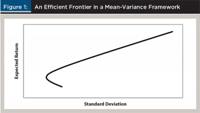
A set of optimal portfolios with the highest expected return for a given risk, or the lowest risk for a given expected return, is called the efficient frontier. Figure 1 plots a generic efficient frontier. A rational investor will not choose a portfolio that lies below or right of the efficient frontier, because the investor can reduce the risk and also increase the expected return at the same time. Depending on the investor’s level of risk aversion, he or she will optimally choose a portfolio on the efficient frontier. If an investor is more risk averse, his or her optimal portfolio will be on the lower left part of the frontier with a lower risk and a lower return. On the other hand, if another investor is more risk tolerant, the portfolio will be on the upper right part of the frontier with a higher risk and a higher return. Since its inception, this mean-variance framework has been widely used by practitioners and investors to allocate wealth among various assets.
Traditional modern portfolio theory is a static model with only one time horizon. This study extends this static model to a dynamic setting in which investors have to decide how to invest over time. This framework can explain why DCA is so popular among investors in spite of the many academic studies claiming that a lump-sum investing strategy is superior.
The approach presented here analyzes both the expected return and the standard deviation, showing that there is a trade-off between these two variables. Although the expected return is higher for lump-sum investing than for DCA, the standard deviation of lump-sum investing is also higher than that of DCA. Depending on an investor’s level of risk aversion, an investor may not want to invest all of his or her money in risky assets at once. Instead, the investor may want to invest equal amounts over time to reduce the risk. Results suggest that despite the fact that it provides a lower return than lump-sum investing, DCA can still be an optimal investment strategy for certain investors.
Literature Review
Constantinides (1979) was the first economist to criticize the use of DCA as a viable investment strategy for minimizing risk in the stock market. Constantinides showed theoretically that DCA is dominated by a sequential optimal investment strategy, which allows for the use of information that becomes available in the future, as well as optimal non-sequential investment strategies. He thus concluded that DCA strategies are suboptimal.
Several studies following Constantinides reached similar conclusions. Knight and Mandell (1993) used graphical analysis, historical stock returns, and Monte Carlo simulations to show that DCA strategies do not provide any advantage over either optimal rebalancing strategies or buy-and-hold strategies. Williams and Bacon (1993) used historical stock returns from 1926 to 1991 to compare the annualized returns of DCA to those of lump-sum investing strategies. Their results showed that two-thirds of the time, the lump-sum investing strategy provided higher returns than the DCA strategy. They thus concluded that because the average return on a stock is higher than the risk-free rate, investors would give up a positive excess return by spreading their stock purchases throughout the year. Furthermore, Thorley (1994) found that, using the Sharpe ratio and the Treynor ratio measures, DCA empirically had lower expected returns and higher risks when compared with a buy-and-hold strategy.
Using a simulation, Rozeff (1994) found that a lump-sum investing strategy provides higher annualized returns when compared to a DCA strategy. He concluded that as long as the stock market has a positive expected risk premium, lump-sum investing is a better investment strategy, because the invested funds will provide more independent returns, thus increasing expected returns and decreasing volatility.
Abeysekera and Rosenbloom (2000) used a Monte Carlo simulation to show that a DCA strategy leads to lower expected returns and lower volatility than a lump-sum investing strategy. For low-volatility stocks, they found that lump-sum investing is better than DCA, whereas for stocks with high volatility, they found that lump-sum investing provides higher returns but greater risk.
Leggio and Lien (2003) criticized the use of the Sharpe ratio in financial studies that recommend DCA as a superior strategy. Using the Sortino ratio and an upside potential performance ratio, they found that a lump-sum investing strategy actually outperforms DCA.
Greenhut (2006) criticized the mathematical illustrations of DCA used in many studies, suggesting that such strategies depend on stock price trends. Greenhut found that in down markets, DCA works best, but when he examined up markets (which represent expected long-term trends), he found that lump-sum investing strategies outperformed DCA strategies. Greenhut pointed out that because an upward market establishes the norm over time, the reason many studies found that other strategies outperform DCA approaches could be explained by the historical upward market trend of stocks.
Using a Monte Carlo simulation, Dubil (2005) found that the expected return from a DCA strategy is 30 percent lower than that of a lump-sum investing strategy. Dubil found that in up markets, a lump-sum investing strategy outperforms a DCA strategy because it results in buying low up front. During down markets, DCA outperforms a lump-sum investing approach because it results in buying later at a lower price.
This paper offers an alternative explanation for the popularity of DCA strategies by using traditional portfolio theory. As will be shown, results from this study indicate that DCA can be an optimal investment strategy. The findings do not directly contradict those of Thorley (1994) and Rozeff (1994). First, it is acknowledged that a lump-sum investing strategy provides a higher return than DCA. Second, in this study, risk was measured by standard deviation, a key factor in portfolio theory. In contrast, Thorley (1994) used the Sharpe and the Treynor ratio, while Rozeff (1994) used an “adjusted risk” measure that reduced the amount of money invested via lump-sum investing in order to make a comparison between lump-sum investing and DCA.
This study shows that investors, depending on their level of risk aversion, may not wish to invest all of their money in stocks at one time, as investing their money over time will reduce the standard deviation of returns.
Methodology
Using a mean-variance analysis, this paper describes portfolios in terms of standard deviation and expected return. Risk-averse investors prefer higher expected returns and a lower standard deviation. Conventional portfolio theory can be used to analyze the portfolio problem in a static setting. Previous analyses clearly show a diversification effect across assets. This paper finds a similar effect in a dynamic setting over time. This paper shows where a DCA strategy fits into a mean-variance analysis when compared to a lump-sum investing strategy.
Consider, for example, an investor with a specific amount to invest in a risky asset over a certain time period, such as the use of an IRA that has a maximum contribution limit for a calendar year. If the investor decides to use a lump-sum investing strategy, he or she will invest everything now. However, if the investor uses a DCA strategy, he or she can invest half now and the other half later. Previous studies have argued that the lump-sum investing outperforms DCA because of higher expected returns. This study analyzes not only the expected return but also the standard deviation and shows that there is indeed a trade-off between these two variables, which become key factors guiding investment decisions.
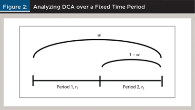
To analyze DCA over a fixed time period, this study looked at two equal-length periods, period 1 and period 2. With this approach, the investor decides on w, or how much to invest at the beginning of period 1 for the entire two periods, versus 1 – w, or how much to defer and invest at the beginning of period 2 for just one period. Thus, w = 100 percent represents a lump-sum investing decision, whereas w = 50 percent represents a DCA strategy, investing equal amounts at the beginning of each period.1 The value of w can range from 0 percent to 100 percent in that the investor can vary the amounts invested now versus later.
We denoted r1 as the period 1 return, and r2 as the period 2 return. We assumed that both periods have the same return distribution. We also assumed the weak-form efficient market hypothesis, which means that returns cannot be predicted and are uncorrelated over time. This resulted in the following mathematically assumptions:
Assumption 1: E(r1) = µ and Var(r1) = σ2.
Assumption 2: E(r2) = µ and Var(r2) = σ2.
Assumption 3: Cov(r1, r2) = 0.
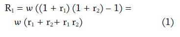
Total return is the sum of two components: (1) the return from investing w for two periods; and (2) the return from deferring (1 – w) to period 2 and investing for one period. First, the return from investing w now for two periods, R1, is
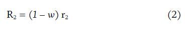
Second, the return from deferring (1 – w) to period 2 and investing for one period, R2, is:
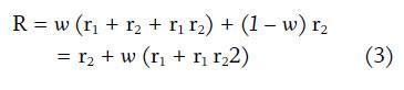
The total return, R, is the sum of R1 and R2, where
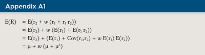
Next, we derived the expected return and the standard deviation of total return, R, to analyze how w, the allocation in period 1, affects these two factors for investment decision-making. First, the expected return is:
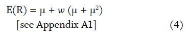
Equation 4 implies that as long as the expected return of the risky asset, µ, is positive, lump-sum investing (w = 100 percent) will outperform DCA (w = 50 percent). This is consistent with the findings of Williams and Bacon (1993), Rozeff (1994), and Abeysekera and Rosenbloom (2000).
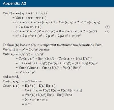
Second, the variance of total return is:
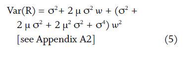
Equation 5 increases with w, which means that a larger investment in period 1 leads to a higher variance and standard deviation. This shows that lump-sum investing (w = 100 percent) is riskier than DCA (w = 50 percent) when standard deviation is used as a measure of risk. As a result, there is a trade-off between risk and return. Even if DCA may result in a lower return, the approach results in a smaller risk than lump-sum investing. This implies that DCA can be superior to lump-sum investing when risk is taken into account for an investor with a high level of risk aversion.
Further analysis of equations 4 and 5 shows that the variance is a quadratic function of the expected return. In other words, the set of investment choices lies on a parabola in mean-variance space. This means the choices can be plotted in a mean-variance two-dimensional graph.
Figure 3 plots the set of investment choices of w, ranging from 0 percent to 100 percent. Given the length of each period is six months, we assumed the expected return of a risky asset (µ) was 4 percent and the standard deviation (σ) was 13 percent for six months. When annualized, this risky asset had an annualized expected return of 8.16 percent and an annualized standard deviation of 19.19 percent, which was similar to the U.S. stock market index.
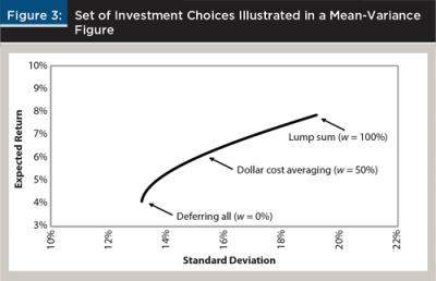
If one invests $0 on the first date and defers all to the second date (w = 0 percent), the expected return is 4 percent and the standard deviation is 13 percent. This corresponds to the left end of the graph in Figure 3. This offers the lowest expected return and the lowest risk among all the investment choices.
Alternatively, if an investor chooses the lump-sum strategy (w = 100 percent) and invests all for the entire year, the expected return is 8.16 percent and the standard deviation is 19.19 percent annualized. This corresponds to the right end of the graph in Figure 3. This offers the highest expected return and the highest risk of all the choices.
We considered the DCA method (w = 50 percent) by investing equal amounts on two dates. This can be thought of as the average between deferring all (w = 0 percent) and lump-sum investing (w = 100 percent). The expected return for the DCA was 6.08 percent using equation 4. This implies that the performance of DCA is the average between deferring the entire investment and lump-sum investing at the outset. The risk of DCA, though, is not the average between the two strategies. From equation 5, the standard deviation of DCA is 14.91 percent. This is smaller than 16.10 percent, which was the average between 13 percent (w = 0 percent) and 19.19 percent (w = 100 percent).
In other words, the risk of DCA is smaller than the average risk between deferring the entire investment and investing a lump-sum at the outset. By diversifying across time, an investor can lower risk. This effect is represented by the parabola shape in Figure 3. This plot may look identical to the standard efficient frontier in Figure 1, but there is a big difference. The standard efficient frontier in Figure 1 is a static model where portfolios are made from a pool of assets in a single period. On the other hand, the set of portfolios in Figure 3 is made from dynamic choices, where an investor decides how much to invest in the first period versus the next period.
We then used a utility function to show how the level of an investor’s risk aversion can affect the optimal investment choice between DCA and lump-sum investing, where
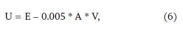
In Equation 6, U is the utility value, E is the expected return, A is the coefficient of risk aversion, and V is the variance of return. Because investors have different levels of risk aversion, A in Equation 6 differs among investors. The higher the A, the more risk averse the investor. The lower the A, the more risk tolerant the investor. Although there may be no standard method to estimate one’s absolute risk aversion, the typical range of coefficients of absolute risk aversion used in the economic literature is between 2 and 4.
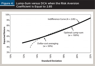
Consider an investor with a risk aversion coefficient of 2.85 who needs to decide between DCA (E = 6.08, V = 14.912) and lump-sum investing (E = 8.16, V = 19.192). The utility scores in equation 6 of both choices are identical at 2.91. This implies that the investor is indifferent between the two choices.2
Figure 4 plots the indifference curve for this investor in the solid line. The indifference curve goes through both investment choices, which means the utility scores are identical to this investor. However, for an investor whose risk aversion coefficient is different from 2.85, the investor will prefer one method to the other. If an investor has a lower risk aversion coefficient than 2.85, the investor will prefer lump-sum investing, because he or she is willing to take more risk for a higher return. However, if an investor has a coefficient greater than 2.85, he or she will prefer a lower risk DCA approach.
Practical Implications and Limitations
Financial planners are often asked to provide investment and tax strategies to their clients. Arguably, one of the most popular tools is an IRA. In contrast with other investment vehicles, the amount to invest in an IRA is not the question for most clients, because IRAs have a maximum contribution limit per calendar year. Instead, the timing of the contribution is a bigger concern. Previous studies have suggested that a DCA strategy is suboptimal because it provides a lower return than a lump-sum investing strategy. The literature implies that financial planners should advise clients to invest the maximum contribution limit as early as possible.
This study compares not only the returns but also the risks between a DCA and a lump-sum investing strategy. Results suggest that there is a trade-off between risk and return. The key practical implication of this finding is that DCA can be an optimal strategy when risk is taken into account. Specifically, investing equal amounts over time is less risky than investing all at once. Accounting for this risk factor, DCA will be optimal for highly risk averse clients.
Two limitations are associated with this study. First, to invest the same amounts in two different dates over time for DCA, we assumed that the deferred amount in period 1 did not earn a risk-free rate of return. If it did, then the investor would invest a different amount in the second period or would leave the earned interest in period 1 not invested in period 2. We investigated both cases and found that the main result of the study—the trade-off between risk and return—does not change. Intuitively, because the risk-free rate has zero variance, the earned interest does not alter the variance of the investment.
Second, we considered two dates to invest in a year. In practice, investors may choose to invest equal amounts more frequently. Having 12 months to invest, for example, instead of two six-month periods, makes the results stronger, not weaker. We showed that investing half of an amount in two different dates over time lowers risk. Investing equal amounts every month will reduce the risk even more. The trade-off between risk and return will persist, and highly risk averse investors should rationally prefer DCA to lump-sum investing.
Conclusion
More than three decades of academic research has shown that DCA is inferior to both lump-sum investing and other investment strategies. Despite these findings, DCA has remained one of the most popular investing methods in practice. Previous studies have tried to attribute the continued popularity of DCA to such factors as behavioral errors, the seasonality of equity returns, high conditional expected returns, and mean reversion in stock prices. Such justifications fall flat and do not satisfactorily explain the wide use of DCA by investors.
This study provides a theoretical justification for the popularity of DCA based on a mean-variance analysis. The study analyzed both the expected return and the standard deviation, showing that there is a trade-off between risk and return, and that these are two key factors instrumental to making an informed investment decision.
Although the expected return was lower for DCA than for lump-sum investing, the risk was also smaller for DCA compared to lump-sum investing. This implies that financial planners should provide DCA advice to their clients who are more risk averse, as investing over time can reduce the risk.
Endnotes
- When w = 50 percent, half the amount is invested first. In order to have the same amount invested later for DCA, the deferred 50 percent remains as cash in period 1 and gets fully invested in period 2. Earning interest on the deferred 50 percent in period 1 does not change the conclusions of the study.
- Instead of choosing between dollar-cost averaging and lump-sum, if this investor could choose any w, the optimal choice would be w = 75 percent.
References
Abeysekera, Sarath P., and E.S. Rosenbloom. 2000. “A Simulation Model for Deciding between Lump-Sum and Dollar-Cost Averaging.” Journal of Financial Planning 13 (6): 86–96.
Atra, Robert J., and Thomas L. Mann. 2001. “Dollar-Cost Averaging and Seasonality: Some International Evidence.” Journal of Financial Planning 14 (7): 98–103.
Brennan, Michael J., Feifei Li, and Walter N. Torous. 2005. “Dollar-Cost Averaging.” Review of Finance 9 (4): 509–535.
Constantinides, George M. 1979. “A Note on the Suboptimality of Dollar-Cost Averaging as an Investment Policy.” Journal of Financial and Quantitative Analysis 14 (2): 443–450.
Dichtl, Hubert, and Wolfgang Drobetz. 2011. “Dollar-Cost Averaging and Prospect Theory Investors: An Explanation for a Popular Investment Strategy.” Journal of Behavioral Finance 12 (3): 41–52.
Dubil, Robert. 2005. “Lifetime Dollar-Cost Averaging: Forget Cost Savings, Think Risk Reduction.” Journal of Financial Planning 18 (10): 86–90.
Greenhut, John G. 2006. “Mathematical Illusion: Why Dollar-Cost Averaging Does Not Work.” Journal of Financial Planning 19 (10): 76–83.
Knight, John R., and Lewis Mandell. 1993. “Nobody Gains from Dollar-Cost Averaging: Analytical, Numerical, and Empirical Results.” Financial Services Review 2 (1): 51–61.
Leggio, Karyl B., and Donald Lien. 2001. “Does Loss Aversion Explain Dollar-Cost Averaging?” Financial Services Review 10 (1–4): 117–127.
Leggio, Karyl B., and Donald Lien. 2003. “Comparing Alternative Investment Strategies Using Risk-Adjusted Performance Measures.” Journal of Financial Planning 16 (1): 82–86.
Markowitz, Harry. 1952. “Portfolio Selection.” Journal of Finance 7 (1): 77–91.
Milevsky, Moshe A., and Steven E. Posner. 2003. “A Continuous-Time Re-examination of the Inefficiency of Dollar-Cost Averaging.” International Journal of Theoretical and Applied Finance 6 (2): 173–194.
Rozeff, Michael S. 1994. “Lump-Sum Investing versus Dollar-Averaging.” Journal of Portfolio Management 20 (2): 45–50.
Statman, Meir. 1995. “A Behavioral Framework for Dollar-Cost Averaging.” Journal of Portfolio Management 22 (1): 70–78.
Thorley, Steven. 1994. “The Fallacy of Dollar-Cost Averaging.” Financial Practice and Education 4 (2): 138–143.
Trainor, William J. 2005. “Within-Horizon Exposure to Loss for Dollar-Cost Averaging and Lump-Sum Investing.” Financial Services Review 14 (4): 319–330.
Williams, Richard E., and Peter W. Bacon. 1993. “Lump-Sum Beats Dollar-Cost Averaging.” Journal of Financial Planning 6 (2): 64–67.
Citation
Cho, David, and Emre Kuvvet. 2015. “Dollar-Cost Averaging: The Trade-Off Between Risk and Return.” Journal of Financial Planning 28 (10): 52–58.