Journal of Financial Planning: October 2013
Jonathan Guyton, CFP®, is principal of Cornerstone Wealth Advisors Inc., a holistic financial planning and wealth management firm in Edina, Minnesota. He is a researcher, mentor, author, and frequent national speaker on retirement planning and asset distribution strategies, and a former winner of the Journal of Financial Planning Call for Papers competition.
Have you ever found yourself perplexed by the potential impact that the pesky problem called sequence-of-returns (SOR) risk can have on a retiree’s portfolio? At times it can seem like the proverbial 800-pound gorilla lurking around the best-laid financial plans.
A common metaphor for SOR risk involves choosing a ball from an urn filled with many identical balls. Each ball announces the inflation rate and returns for the portfolio’s holdings or asset classes for the year. The risk to a client’s retirement income plan comes from the chance of having a number of bad draws in the first four to six years. Therein lies the pesky part: there’s nothing you can do about luck of the draw.
This is a major reason why most sustainable withdrawal rate research can’t compute a more generous result at high levels of success. (Another reason is the risk of abnormally high inflation early on.) There’s always that chance of bad returns in the first few years, and you can’t do anything about that. Or so the research assumes. And so it is often understood to be. This is what I want to explore.
Checking in on the Year 2000 Retiree
Quantifying the potential impact of SOR risk on sustainable withdrawal rates and/or underlying portfolio values typically involves comparing what happens when a specific return and inflation sequence over a period of years is reversed. We know that, mathematically, the average annual return (arithmetic and geometric) is the same regardless of the order of these yearly returns. Such SOR comparisons involve annual rebalancing to a target asset allocation and increases in each year’s withdrawal amount by the prior year’s inflation rate. Thus, any differences in the resulting pair of sustainable withdrawal rates or probabilities of success or ending portfolio values can be laid at the hairy gorilla feet of the sequence itself.
The case of the year 2000 retiree, now in its 14th year of distributions, is especially intriguing for such a comparison. It has been suggested that this real-life retirement date could be the one that ultimately fails despite following the well-known “rules” for generating sustainable withdrawals. We don’t yet know, but, a year 2000 retiree is now almost halfway through a 30-year distribution period.
From a SOR risk perspective, this is a juicy time to check on how things are going. Starting in 2000, a retiree experienced equity returns of –9.5 percent, –13.6 percent, and –19.6 percent in the first three years using a blended index of 2/3 Russell Global and 1/3 Russell 3000. (This produces an allocation of about 65 percent U.S. equities.) These are not the equity returns one wants right out of
the gate!
The first three years of reverse-order returns from 2012, 2011, and 2010 are +16.9 percent, –4.4 percent, and +15.8 percent. Such a difference seems to create the circumstances for SOR risk to wreak havoc. And so it does, at least when the portfolio is rebalanced to the same allocation and the withdrawal amount is increased by inflation in each year.
Static Approach
Table 1 summarizes the results of a static-policy approach. I use a $1.2 million starting value because a year 2000 retiree with a $1 million retirement goal actually accumulated a 20 percent to 25 percent larger nest egg than would have been reasonably projected just four years earlier. A $48,000 (4 percent) initial withdrawal amount is increased annually by the prior year’s inflation (CPI). The portfolio is rebalanced annually to a 60/40 equity/fixed allocation using the blended equity index described above; the fixed income allocation is represented by the same Barclays Intermediate U.S. Government Bond Index used in most prior withdrawal rate research. This static rebalancing policy produces the same 4.7 percent average annual return in both 13-year return sequences; not great, but seemingly not a problem either.
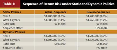
However, there is a large difference—more than 16 percent—in total portfolio value available to generate yearly distributions during the second half of retirement. With the actual sequence, the withdrawal rate for year 14 has grown to 6.1 percent—more than a 50 percent increase from its start. In the reverse-order sequence, the withdrawal rate is now 5.2 percent, “only” a 30 percent increase. Viewing this difference from another perspective, a year 2000 retiree now has about 10 percent less money than when she retired, compared to having 5 percent more than her starting value with the reversed sequence.
Something beyond the year 2000 retiree’s control is likely making a difference in how she views her future financial security. It also could affect the advice she now receives from her financial planner. Or both.
Dynamic Approach
For a healthier financial situation, employ dynamic, rather than static, policies to guide annual decision-making about the asset allocation and distribution amount. Using dynamic policies such as those suggested in the published works of Guyton, Guyton and Klinger, or Bengen, as well as the dynamic allocation policies as developed by Kitces, Pfau, or Gupta et al., we can conduct a similar analysis of the same SOR environment.
In the analysis, I use the dynamic withdrawal policies in Guyton and Klinger (2006) that can trigger a freeze in the distribution amount following years with negative investment returns or a 10 percent real cut (raise) if the withdrawal rate rises (falls) more than 20 percent from its initial percentage.
For the dynamic allocation policies, I use the threshold in Gupta et al. (2012), which relies on the Shiller Cyclically-Adjusted Price/Earnings (CAPE) ratio to gauge market valuation level. The dynamic allocation policy research mentioned above triggers rather large changes to the equity allocation when over-valued or under-valued situations occur.
Gupta et al. (2012) and Pfau (2012) start with a 50 percent neutral equity allocation and decrease (increase) it by half to 25 percent (75 percent) when markets become over- (under-) valued; Kitces employs a smaller adjustment via a 60 percent neutral equity allocation that falls (rises) by one-third to 40 percent (80 percent) when triggered.
Because of my sense that most financial planners (including myself) may be uncomfortable communicating so large a one-time equity allocation change to their clients, in modeling the dynamic allocation policy I use a 65 percent neutral equity allocation with just under a 25 percent shift to 50 percent (80 percent) when an over- (under-) valuation occurs.
Though exhaustive study on the combined impact of dynamic withdrawal and allocation policies has yet to be undertaken, results of their stand-alone impact offer strong reason to believe that employing them together would add around 100 basis points to the sustainable withdrawal rate under static policies. Thus, the year 2000 retiree following such policies can begin by taking a $60,000 (5 percent) distribution. (A different approach would be to designate $100,000 as a discretionary fund and begin with a $55,000 distribution from the remaining $1.1 million core portfolio.)
The results of implementing both dynamic policies simultaneously are striking. Under the actual return sequence, the year 2000 retiree begins her 14th year of distributions with a 9 percent larger nest egg than when she retired. Her next year’s withdrawal amount following the inflationary increase will be 5 percent of the portfolio’s value. Under the dynamic withdrawal policies, she previously had one freeze after 2001 and two cuts after 2002 and 2008.
The dynamic allocation policies produced a 6.3 percent average annual return during the first 13 years of her retirement. In six different years (2000–2002, 2007–2008 and 2011), the equity allocation was reduced to 50 percent due to market over-valuation. Compared with results from the static policy approach, the year 2000 retiree now has 20 percent more assets and has taken nearly 10 percent more in distributions. Twice, she had to adjust to two years with modest (3 percent to 5 percent) declines in her total spendable income, but she was far less likely to be faced with the stress of deciding whether a significant lifestyle change was necessary.
Lessening the Impact of SOR
What about the impact of the return sequence with these dynamic policies in place? Before discussing the results, I must make several comments about modeling the reverse-order SOR under the dynamic policies.
Determining the next year’s withdrawal amount via the withdrawal policies was straightforward when knowing the prior year’s ending value, return, and inflation. However, employing the allocation policies was somewhat subjective because the earnings portion of the CAPE ratio would not necessarily flow seamlessly in reverse-order with its numerator. Therefore, I chose to let the most recent equity returns guide the valuation assessment and resolve uncertainties in the direction more favorable to helping the reverse-order SOR result.
For example, after averaging 9 percent over the first three reverse-order years (2012–2010), equities could have been considered over-valued and reduced to 50 percent just before the next year’s large gain (2009); I did not do this until prior to the following year. All-in-all, equities under reverse-order SOR were deemed over-valued four times. Because they never reached under-valued status in the actual SOR, they did not in the reverse-order SOR either. Its annualized return was a very similar 6.1 percent.
When using the dynamic withdrawal and allocation policies, the SOR impact is far less noticeable. As expected, the reverse-order SOR generated a higher portfolio value after 13 years, but only 1 percent higher. Total distributions were about 5 percent higher as the reverse-order SOR scenario had one more year with an inflationary increase (no cuts and two freezes) under the dynamic withdrawal policies. In this comparison, both sets of dynamic policies made a contribution.
This analysis of a single 13-year period is far from sufficient to claim that the combined application of dynamic withdrawal and allocation policies makes the often-feared SOR risk more like a boogeyman in the closet than an 800-pound gorilla in the room. However, it can serve as a compelling Exhibit A.
Not only can these dynamic policies trigger the mid-course adjustments occasionally required in a sustainable distribution strategy with a higher initial withdrawal rate, their empowering ongoing application can go a long way in blunting the impact of those economic circumstances that lie beyond our control.
References
Bengen, William P. 2006. Conserving Client Portfolios During Retirement. Denver: FPA Press.
Gupta, Neeraj J., Robert Pavlik, and Wonhi Synn. 2012. “Adding ‘Value’ to Sustainable Post-Retirement Portfolios.” Financial Services Review (spring).
Guyton, Jonathan T. 2004. “Decision Rules and Portfolio Management for Retirees: Is the ‘Safe’ Initial Withdrawal Rate Too Safe?” Journal of Financial Planning 17, 10 (October): 54–62.
Guyton, Jonathan T., and William J. Klinger. 2006. “Decision Rules and Maximum Initial Withdrawal Rates.” Journal of Financial Planning 19 (3): 48–58.
Kitces, Michael E. 2009. “Dynamic Asset Allocation and Safe Withdrawal Rates.” The Kitces Report (April).
Pfau, Wade D. 2012. “Withdrawal Rates, Savings Rates, and Valuation-Based Asset Allocation.” Journal of Financial Planning 25 (4): 34–52.