Journal of Financial Planning: November 2011
Executive Summary
- This paper presents a new measure of active fund performance that evaluates funds in a manner aligned with what investors seek to optimize: utility.
- Unlike the information ratio, currently one of the most popular metrics of performance used by practitioners, this measure assumes a concave utility function and incorporates risk aversion.
- The importance of these improvements is conveyed through comparative static analysis.
- Using a sample of mutual funds, this paper shows the differences in rankings of funds derived through the use of the new measure rather than the information ratio.
David Nanigian, Ph.D., is an assistant professor of investments at The American College.
The purpose of this paper is to describe a new measure of actively managed fund performance grounded in utility theory. Currently, practitioners consider the information ratio (IR), developed by Treynor and Black (1973), one of the most important metrics of fund performance as discussed in Grinold (1989) and Menchero (2006/2007). The general version of the IR is simply the ratio of return in excess of a benchmark index divided by the volatility of the excess returns. As explained in Menchero (2006/2007), the specialized model typically employed by financial services professionals is specified as:
where BAR denotes benchmark-adjusted return and TEV denotes tracking error volatility. Benchmark-adjusted return is the time-series raw mean difference between a fund’s net returns and the returns on its respective benchmark index. Tracking error volatility is the time-series standard deviation of the difference between a fund’s net returns and the returns on its benchmark index. An insightful discussion of the IR can be found in Goodwin (1998).
The advantages of the IR lie in its computational simplicity and mathematical similarity to Sharpe’s (1966) reward-to-variability ratio, a more general measure of investment performance. Two important assumptions of the IR are that the utility one derives from changes to wealth is irrespective of his or her level of wealth and that investors have identical levels of risk aversion. If these assumptions were true, then the IR should play an integral role in the performance evaluation process. However, motivated by Arrow’s (1965) theory of risk-bearing, Kahneman and Tversky (1979) provide empirical evidence that the marginal utility derived from wealth is decreasing in gains to wealth. Additionally, many empirical studies show substantial differences in the level of risk aversion across individuals.1 Evidence in support of non-linear utility functions and different levels of risk aversion among individuals motivates the need for a measure of mutual fund performance that incorporates these characteristics of investor behavior.
The contribution of this article is to put forward the difference between the utility derived from investing in an actively managed fund and the utility derived from investing in a comparable passively managed fund as an alternative measure of fund performance. First, I begin with a description of my measure. Next, I examine how differently funds are ranked when using it as opposed to the IR. Finally, I conclude with practical implications for personal financial planners.
Utility Theory
Utility theory, pioneered by Von Neumann and Morgenstern (1947), implies that under the simplifying assumption of constant relative risk aversion, investors possess the following mean-variance utility function:
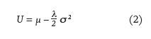
where µ denotes the mean return of an investor’s portfolio, l denotes the investor’s own level of risk aversion, and s 2 denotes the variance of the returns on the investor’s portfolio. From Equation 2, three directional effects are apparent. First, U is increasing in returns. Second, U is decreasing at an increasing rate in s. Third, DU resulting from a given level of s is determined by l. It is quite clear that the second and third effects are absent from the IR, and it should be noted that Israelsen (2005) also expresses concern about the absence of utility theory in IR. These deficiencies motivate the need for a more informative measure of the performance of an actively managed fund.
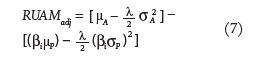
Drawing upon Equation 2, I suggest the following measure of fund performance, which I will refer to as the relative utility of active management measure (RUAM):
where µA denotes the mean return of a given actively managed fund under consideration, and µP denotes the mean return on that fund’s benchmark index over the same time period. δ2A denotes the variance of returns on the actively managed fund, and δ2P denotes the variance of returns on that fund’s benchmark index over the same period. RUAM can be interpreted as a measure of the performance of a given actively managed fund relative to a comparable index fund, and positive values are preferred by investors. In today’s market, there is a plethora of indexed products available to individual investors. Therefore, as detailed in Cremers and Petajisto (2009), it is important to compare a fund’s performance with that of a benchmark index, as products tracking it are always close substitutes.
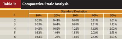
In comparing my measure with the IR, it is similar in that it involves only basic mathematics and is simple to compute. However, it is different in two regards. First, it allows an investor to evaluate the performance of fund managers based on his or her own risk preference. Second, its assumption of decreasing rather than constant marginal utility from wealth is more consistent with utility theory and investor behavior. Table 1 conveys comparative-static results of the impact of a one percentage point increase in δ at various parameters of λ and δ on U. The table clearly highlights the importance of incorporating one’s own risk preference and the decreasing marginal utility from wealth into the performance evaluation framework. For example, ΔU associated with a one percentage point increase in δ is 50 percent greater for an investor with λ = 3 than for one with λ = 2, and ΔU associated with a one percentage point increase in δ is nearly twice as great for an asset with a δ of 20 percent than one with a s of 10 percent. It should be noted that Goetzmann, Ingersoll, Spiegel, and Welch (2007) developed a measure similar to mine in many respects, but it only examines funds in isolation; that is, it doesn’t compare their performance to a benchmark, and it is more mathematically complex.
Data
Because there is time variation in IRs, I follow Bossert, Fuss, Rindler, and Schneider (2010) and calculate performance metrics over a one-year interval. My sample period spans January 4, 2010, through December 31, 2010.2 Weekly return data on individual mutual funds and benchmark indices as well as mutual fund total net assets data come from Morningstar Direct. The selection of a weekly frequency was also motivated by Bossert, Fuss, Rindler, and Schneider (2010), as they find that it not only allows for a sufficient sample size from which to estimate standard deviations over a one-year interval but also produces results similar to those obtained from higher frequency data.
My initial sample consists of all open-end mutual funds domiciled in the United States with a U.S. broad asset class of “U.S. stock.” Because the purpose of this paper is to focus on the value added by active management to individual investors’ portfolios, index funds, enhanced index funds, and institutional funds are excluded from analysis.
The question of which benchmark is most appropriate for performance evaluation is one of considerable debate. One commonly agreed-upon attribute, however, is that the role of a benchmark in the performance evaluation process is to separate returns attributable to common risk factors from those attributable to managerial skill. See, for example, Rennie and Cowhey (1990) and Kritzman (1987) for a discussion of this.
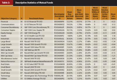
Sensoy (2009) finds that about one-third of mutual funds, as stated in the prospectus, have benchmarks that do not match their style, and he provides a compelling argument in favor of funds purposely comparing themselves with benchmarks that offer relatively low returns in order to attract investors. Therefore, I compare funds with the performance of their benchmarks as assigned by Morningstar’s analysts rather than as stated in the prospectus. This is because Morningstar mainly considers the recent portfolio holdings of a mutual fund in its assignment of a fund to an objective category and then to a benchmark.3 The benchmarks associated with each objective category are conveyed in Table 2. It should also be noted that I used the “include all investments” as opposed to the “include only surviving investments” option from Morningstar Direct in order to prevent surviving funds from upwardly biasing my results.
Share-class returns are always weighted by month-end total net assets (TNA). In the event a week spans two months, the data are weighted by TNA as of the month in which the week ended. Funds lacking 52 weeks of continuous (fund-level) return data to calculate metrics of performance are omitted. My final sample consists of 2,269 funds.
Results
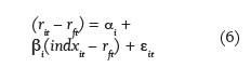
Descriptive Statistics. Table 2 provides descriptive statistics on each of the objective categories in my study. Returns and standard deviations are annualized to facilitate ease of interpretation. Standard deviations are annualized through multiplying them by a factor of √ 52 . Returns are annualized through the use of buy-and-hold returns (BHR) and are calculated by compounding the weekly returns over the time-series. Buy-and-hold abnormal returns (BHAR) are the difference between the returns on a fund and that of its benchmark index, that is,
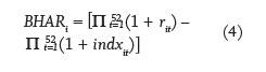
where rit denotes the return on fund i in month t and indxit denotes the contemporaneous return on that fund’s benchmark index.
My sample is somewhat dominated by large-cap funds, with funds in either the large-blend, large-growth, or large-value objective categories making up half of the sample. Over the period of analysis, the mean return across all funds in each objective category was positive, yet BHAR, IR, and RUAM (when evaluated at λ = 3 and λ = 5) all present mixed results on the performance of funds net of their benchmarks.
Sensitivity of RUAM to Risk Aversion Levels. One of the unique features of RUAM is its use of l as an input. Although the comparative-static results of ΔU shown in Table 1 suggest that λ may meaningfully affect investment decisions obtained through the use of RUAM in this section, I examine whether this postulation is supported by the data.
To examine the importance λ plays as an input in RUAM, I compile the distribution of all funds in my sample along two dimensions: quintile of RUAM within objective category when λ = 3 and quintile of RUAM when λ = 5. Table 3 presents these results. The use of quintile rank within objective category rather than quintile rank in the entire cross-section of funds was motivated by Israelsen’s (2005) discussion on how the IR should only be used to rank funds within a particular objective category.
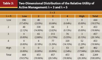
Unsurprisingly, a positive correlation exists between the measures with heterogeneous λ parameters. However, within all quintiles of a given RUAM category, there is considerable variation in the other. For example, 32 percent of funds in the median (third) quintile of one RUAM specification did not rank in the median quintile of the other. Such high sensitivity to λ lends support to the belief that λ is an important determinant of RUAM. Analysis was also conducted using other λ specifications, and the results were similar.
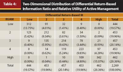
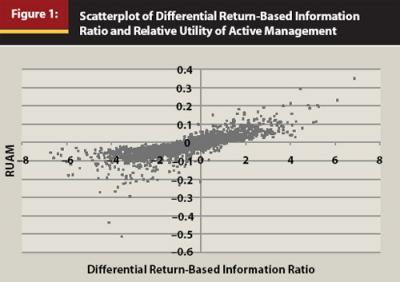
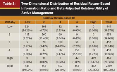
Ranking Funds Through RUAM Versus the IR. In assessing the value of RUAM to financial services practitioners, it is important to gauge not only the sensitivity of the measure to λ but also the difference in one’s assessment of a fund when RUAM is used rather than the IR. Table 4 presents the distribution of all funds in my sample along the dimensions of quintile of the IR and quintile of RUAM when evaluated at λ = 4. The correlation structure is similar to that observed in Table 3, characterized by a positive correlation between the performance rankings provided by the measures, yet considerable variability exists in the rankings. At most, 74 percent of funds in a given quintile of RUAM lie in the same quintile of the IR. The differences between the IR and RUAM are graphically represented in Figure 1.
As can be inferred from Equation 1, practitioners do not typically adjust for a fund’s beta when deriving its IR. However, Roll (1992) and Jorion (2003) explain that this myopic framework of performance evaluation incentivizes fund managers to leverage up their funds. Therefore, I also adjust both the IR and RUAM for the beta from a single-index model regression of the excess returns of a fund on those of its benchmark index. Following Amihud and Goyenko (2010), I employ the following alternative specification of the IR:
where αi is the intercept and RMSEi is the squared root of the mean-squared errors from a single-index regression model, specified as:
where rft denotes the risk-free rate of interest, proxied by the average of business days’ secondary-market rate on four-week Treasury bills. The time-series of Treasury yields is gathered from Federal Reserve Economic Data. I also adjust both µP and sP in RUAM by βi. More formally,
The results from Equations 5 and 7 are shown in Table 5. When comparing these results with those obtained through the prior comparison of differential return-based IR and unadjusted RUAM there is somewhat less disparity in the rankings of funds after adjusting for beta. However, it is clear that one’s evaluation of a fund may still be considerably altered through the use of RUAM.
Conclusion
The purpose of this paper was to describe a new measure that allows a financial planner to evaluate the performance of actively managed funds in a manner consistent with utility theory and the behavior of individual investors. Unlike the information ratio, currently one of the most popular metrics of performance used by practitioners, my measure assumes a concave utility function and incorporates risk aversion. Comparative static analysis conveys the importance of these improvements. I also analyze a sample of 2,269 U.S. equity mutual funds and show there are considerable differences between the rankings of funds derived through the use of RUAM and those derived through the use of the IR. Moreover, the measure is easy for a financial planner to calculate, as it requires only an estimate of his or her client’s level of risk aversion, a time-series of returns on a fund and its benchmark index, and a basic knowledge of arithmetic.
Motivated by Jorion’s (2003) compelling argument in favor of analyzing a fund in the context of an investor’s total portfolio, it would be interesting to apply the measure described in this paper to the total portfolio setting through an alternative specification of the inputs in its formula. For example, if an investor has some portion of his or her portfolio allocated to a particular asset class, one could compute the return and standard deviation on that investor’s total portfolio under the scenario that all funds allocated to the asset class are placed in a given active fund. Then, one could derive the associated utility score, do the same under the alternative scenario that funds allocated to the asset class under consideration are passively managed, and compare the two scores. Such analysis will consider the correlation structure of asset returns in an investor’s portfolio and is a ripe topic for future research.
Endnotes
- See, for example, Holt and Laury (2002); Bakshi and Madan (2006); Choi, Fisman, Gale, and Kariv (2007); Andersen, Harrison, Lau, and Rutstrom (2008); and Harrison, Lau, and Rutstrom (2009) for evidence on heterogeneous levels of risk aversion in the cross-section of market participants.
- In the interest of dismissing concerns of “data snooping,” I also conduct my empirical analysis over 2009. The results were similar to those obtained over 2010.
- Details on the methodology employed by Morningstar to assign a fund to an objective category can be found at http://corporate.morningstar.com/us/documents/Methodology Documents/MethodologyPapers/Morningstar Category_Classifications.pdf.
References
Amihud, Y., and R. Goyenko. 2010. “Mutual Fund’s R² as Predictor of Performance.” New York University Working Paper No. FIN-08-046.
Andersen, S., G. W. Harrison, M. I. Lau, and E. E. Rutstrom. 2008. “Eliciting Risk and Time Preferences.” Econometrica 76, 3: 583–618.
Arrow, K. J. 1965. Aspects on the Theory of Risk Bearing. Helsinki: Yrjo Hahnsson Foundation.
Bakshi, G., and D. Madan. 2006. “The Distribution of Risk Aversion.” University of Maryland Smith School of Business Working Paper.
Bossert, T., R. Fuss, P. Rindler, and C. Schneider. 2010. “How ‘Informative’ Is the Information Ratio for Evaluating Mutual Fund Managers?” Journal of Investing 19, 1: 67–81.
Choi, S., R. Fisman, D. Gale, and S. Kariv. 2007. “Consistency and Heterogeneity of Individual Behavior Under Uncertainty.” American Economic Review 97, 5: 1921–1938.
Cremers, M., and A. Petajisto. 2009. “How Active Is Your Fund Manager? A New Measure That Predicts Performance.” Review of Financial Studies 22, 9: 3329–3365.
Goetzmann, W., J. Ingersoll, M. Spiegel, and I. Welch. 2007. “Portfolio Performance Manipulation and Manipulation-Proof Performance Measures.” Review of Financial Studies 20, 5: 1503–1546.
Goodwin, T. H. 1998. “The Information Ratio.” Financial Analysts Journal 54, 4: 34–43.
Grinold, R. 1989. “The Fundamental Law of Active Management.” Journal of Portfolio Management 15, 3: 30–37.
Harrison, G. W., M. I. Lau, and E. E. Rutstrom. 2009. “Risk Attitudes, Randomization to Treatment, and Self-Selection into Experiments.” Journal of Economic Behavior and Organization 70, 3: 498–507.
Holt, C. A., and S. K. Laury. 2002. “Risk Aversion and Incentive Effects.” American Economic Review 92, 5: 1644–1655.
Israelsen, C. L. 2005. “A Refinement to the Sharpe Ratio and Information Ratio.” Journal of Asset Management 5, 6: 423–427.
Jorion, P. 2003. “Portfolio Optimization with Tracking-Error Constraints.” Financial Analysts Journal 59, 5: 70–82.
Kahneman, D., and A. Tversky. 1979. “Prospect Theory: An Analysis of Decision Under Risk.” Econometrica 47, 2: 263–292.
Kritzman, M. 1987. “Incentive Fees: Some Problems and Some Solutions.” Financial Analysts Journal 43, 1: 21–26.
Menchero, J. 2006/2007. “Risk-Adjusted Performance Attribution.” Journal of Performance Measurement: 22–28.
Rennie, E. P., and T. J. Cowhey. 1990. “The Successful Use of Benchmark Portfolios: A Case Study.” Financial Analysts Journal 46, 5: 18–26.
Roll, R. 1992. “A Mean/Variance Analysis of Tracking Error.” Journal of Portfolio Management 18, 4: 13–22.
Sensoy, B. A. 2009. “Performance Evaluation and Self-Designated Benchmark Indexes in the Mutual Fund Industry.” Journal of Financial Economics 92, 1: 25–39.
Sharpe, W. F. 1966. “Mutual Fund Performance.” Journal of Business 39, 1: 119–138.
Treynor, J. L., and F. Black. 1973. “How to Use Security Analysis to Improve Portfolio Selection.” Journal of Business 46, 1: 66–86.
Von Neumann, J., and O. Morgenstern. 1947. Theory of Games and Economic Behavior. 2nd ed. Princeton, NJ: Princeton University Press.
Acknowledgments: The author appreciates the feedback given by an anonymous reviewer and by seminar participants at The American College.