Probability-of-Failure-Based Decision Rules to Manage Sequence Risk in Retirement

Journal of Financial Planning: November 2011

Executive Summary

• This paper demonstrates how practitioners can better use the often-overlooked probability of failure as a decision tool.
• Withdrawal rates depend on the retiree’s age (distribution time remaining), and therefore withdrawal rates alone do not tell a complete sustainable distribution story.
• Probability of failure does not depend on the retiree’s age and is therefore useful for comparison of withdrawal rates over any time period or asset allocation.
• Comparison of probability-of-failure curves, and their shift between strategies, illustrates how effective one strategy is compared with another.
• The methodology presented provides an ability to evaluate the withdrawal rate and exposure to sequence risk together.
• This paper seeks to answer the question: how can you determine when a withdrawal rate is too high, as well as subject to poor (or good) markets as the retiree ages?
• The paper concludes with practical applications for practitioners from two key insights: (1) results from a prior simulation would be different for a current simulation (different transient states as defined in the paper), and (2) a range of probability of failure is desired over trying to maintain a steady probability of failure.

Larry R. Frank Sr., CFP^®, is a registered investment adviser in Rocklin, California.

John B. Mitchell, D.B.A., is professor of finance at Central Michigan University.

David M. Blanchett, CFP^®, CLU, AIFA^®, QPA, CFA, is the director of consulting and investment research for the Retirement Plan Consulting Group at Unified Trust Company in Lexington, Kentucky.

Past research on sustainable withdrawal rates has focused primarily on static simulations based on the perspective of an “initial,” or safe, sustainable withdrawal rate. This approach ignores the fact that the variables affecting retirement income are dynamic over time. This has been demonstrated by recent market upheavals, which have caused many practitioners to question the long-term sustainability of withdrawal strategies. In this paper, the authors demonstrate a methodology in which the withdrawal dollar amount dynamically adjusts as the retiree ages.¹

This dynamic concept is captured using the term “current” as opposed to “initial.” This becomes an iterative process as the retiree continues to age and the other variables subsequently also change over time.

Past research has tended to focus on safe withdrawal rates combined with withdrawal-rate-based decision rules; see for example Guyton (2004), Guyton and Klinger (2006), Pye (2008), Stout (2008), and Mitchell (2011). If the retiree continues to strive to maximize withdrawals as he or she ages, a result is increased exposure to sequence risk. This problem is exacerbated by unpredictable, significant market movements (black swans) as discussed by Mandelbrot and Hudson (2004) and Taleb (2007). The challenge is to manage both withdrawal sustainability and ever-present sequence risk (Frank and Blanchett 2010) when adverse events occur (for example, market declines or unexpected, large required withdrawals).

The problem with a withdrawal rate approach is that the withdrawal rate alone does not directly inform the observer whether ruin is imminent for the (unknown) time remaining; hence, various past researchers established decision rules to manage this exposure to sequence risk. Research by Blanchett and Frank (2009) suggests that withdrawal rates are relatively “low” for longer planning horizons, but increase as the retiree’s distribution period shortens (as he or she ages). Thus, withdrawal rates are time-dependent (values that change as the retiree ages), and therefore are not useful variables when making sequence risk decisions. This paper demonstrates a methodology for evaluating the use of probability of failure, a time-independent variable (values do not change as the retiree ages).

The retirement distribution problem is a function of four variables that can be plotted three-dimensionally: time, withdrawal rate percentage, portfolio allocation, and probability of failure (POF). Our hypothesis is that probability-of-failure-based decision rules can be developed to warn a retiree that adverse return sequences may put distributions at risk of depletion within his or her lifetime. With such a warning, these same decision rules may suggest a method for practitioners to adjust either the portfolio allocation and/or withdrawal amount to avoid running out of money before the retiree’s death. This paper uses fixed distribution periods. A future paper by the authors will integrate longevity with the methodology presented here.

The point of reference for Guyton-type decision rules is based on an initial withdrawal rate. This is, by definition, a time reference to some point in the past. But what past time point is relevant for this decision? This paper shifts the point of reference for decision rules into the future by using a future-oriented reference point for the time function. Therefore, this paper always uses current withdrawal rates as opposed to a previous initial, or safe, withdrawal rate perspective.

The previously retired person who may have experienced portfolio value decline and hence seen his current withdrawal rates go up (even though his initial withdrawal rate from a previous simulation may suggest they were fine), needs to decide when to retrench spending to the level suggested for new retirees. This paper provides guidelines for withdrawal management specifically as a result of variable portfolio values from market sequences.

Asset Classes, Time Sequencing, and Simulation Periods

Monthly real returns for the five asset classes shown below were collected from January 1926 through December 2010. Inflation is measured by the increase in the Consumer Price Index for Urban Consumers, data obtained from the Bureau of Labor Statistics.

• Cash: 30-day T-bill
• Bond: Ibbotson Associates Long-Term Corporate Bond Index
• Domestic large-cap equity: S&P 500
• Domestic small-cap equity: Ibbotson Associates U.S. Small Stock Index
• International large-cap equity: Global Financial Data Global ex USA Index from January 1926 to December 1969; MSCI EAFE from January 1970 to December 2009

Portfolios are assumed to be composed of cash/fixed and equity. The cash/fixed component is 25 percent cash and 75 percent bond. The equity component is 50 percent domestic large-cap equity, 25 percent domestic small-cap equity, and 25 percent international large-cap equity. For example, a 60/40 portfolio (60 percent equity and 40 percent cash/fixed) would be composed of 10 percent cash, 30 percent bond, 30 percent domestic large-cap equity, 15 percent domestic small-cap equity, and 15 percent international large-cap equity.

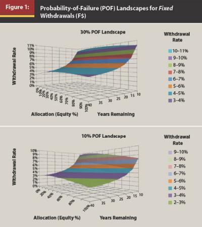
Simulation distribution periods in Figure 1 are 40 through 10 years, in one-year increments. The purpose of this first step in the investigation is to parse out where probability-of-failure landscapes plot (0–5 percent landscape, 5.1–10 percent landscape, etc.), which is a new approach.

Probability of Failure Serves as a Baseline for Subsequent Comparison

Step 1 generates fixed-withdrawal-rate data (Figure 1) to provide the baseline data for subsequent strategy comparisons. Fixed real (inflation-adjusted) distributions are taken from the portfolio at the beginning of each year in a 10,000-run Monte Carlo generator. Probability of failure is defined as the percentage of portfolios with negative values at the end of the planning horizon.

The withdrawal rate problem is three-dimensional. A dynamic approach investigates changes along all three axes simultaneously. Most research consists primarily of keeping the allocation within a single static asset allocation for the duration of the distribution time. Little research (see Garrison, Sera, and Cribbs 2010 for a recent exception) has explored the dynamic effect of changing the portfolio allocation within the simulation, as has been done for dynamically changing withdrawal rates within the simulation over time (Blanchett and Frank 2009).

All points graphed in Figure 1 have the same approximate probability-of-failure rate throughout the same probability-of-failure landscape. Higher probability-of-failure landscapes would map out higher on the withdrawal rate axis because corresponding withdrawal rates are higher; that is, the 5 percent probability-of-failure landscape would lie under the 20 percent probability-of-failure landscape, which in turn is below the 30 percent probability-of-failure landscape for all periods and asset allocations. Note that as distribution time shortens, withdrawal rates may increase, all with a similar approximate exposure to probability of failure. For example, with 60 percent equity allocation, a 3.5 percent withdrawal rate is possible for 30 years, and a 6.05 percent withdrawal rate is possible for 15 years, both with a 10 percent probability of failure; correspondingly, withdrawal rates of 4.75 percent for 30 years and 7.6 percent for 15 years co-exist on the 30 percent probability-of-failure landscape.

Figure 2 shows four cross-sections of Figure 1 at various distribution periods to illustrate longer-term distributions for early retirees (35 years), mid-term periods (25 and 20 years), and a short-term distribution period (10 years) for older retirees (all other cross-sections co-exist throughout the time-remaining axis). These sample cross-sectional views through the probability-of-failure landscapes allow better visualization of how the withdrawal rates with the same probability of failure shift up as distribution time shortens. Consistent tendencies also emerge as to asset allocations.

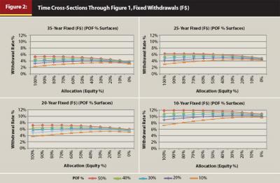
Stopping the illustrations at any particular probability of failure is arbitrary (the authors stop illustration at 50 percent probability of failure). Probability-of-failure landscapes exist along the full spectrum between 0 to 100 percent.

This paper extends previous research in order to answer the following questions: what are more refined decision rules for a retiree? At what withdrawal rate does a retiree need to reduce his withdrawal amount? More importantly, is a single “withdrawal-rate-adjustment rule” true at any probability of failure, time period, or asset allocation? These are questions the practitioner needs to be able to answer.

Past research has usually stopped at this point without a good answer as to when the withdrawal rate may be excessive. Additional comparative data are required to properly address this issue.

The objective of our research is to separate out two strategies over which a retiree has any real control: (1) changing the asset allocation, or (2) changing the withdrawal amount. The final step is to determine what decision rules emerge to aid distribution decisions as the retiree continues to encounter sequence risk, positive or negative, throughout retirement. In summary, Step 1 established a baseline upon which to compare subsequent research Steps 2 and 3 in order to develop a decision-rule regime.

Recall the fundamental withdrawal rate equation: withdrawal rate equals the withdrawal dollar amount divided by the portfolio value. Because portfolio values fluctuate as a result of market sequences, a retiree’s withdrawal rate fluctuates inversely to portfolio value; hence, probability of failure fluctuates along with the withdrawal rate. This dynamic suggests that a practical application would be to accept a range of acceptable probability of failure. At any particular probability of failure, as portfolio value shrinks from a bad market sequence, probability of failure would increase, but may not yet require a retrenchment decision to remain at a reasonable risk level. Is there a maximum probability of failure at which a retiree must retrench spending or face runaway risk? The high end of the probability-of-failure range emerges from data in Step 2.

Transient States

The above baseline data set represents starting a fixed withdrawal at each moment in time and is developed in order to evaluate and compare strategies. Although the simulations are run with fixed withdrawals, in reality each simulation data point is transient depending on factors beyond the retirees’ control: (1) the decreasing time remaining for the retirees’ distribution as they age (Blanchett and Frank 2009, Frank and Blanchett 2010) and (2) the portfolio value.

Practitioners tend to think in terms of simulations and project a single result (the “safe withdrawal rate”) “forever” into the future. However, in truth, simulations or calculations are projected results representing only that single point in time, which is in a transient state. If we run a simulation at time T₁, we get a certain single result. However, the variables change as time passes. Later, at time T₂, when for example the market has declined 5 percent, we run another simulation and get a different single result. The same occurs at time T₃, when the market is now down 10 percent relative to T₁. The same process continues to happen as long as the market declines at each period. All of these results are correct for their given conditions. Should the market recover, the reverse occurs. So practitioners need to look not only at probability-of-failure decision points while the market deteriorates but also at decision points to reverse the process as the market recovers.

Each data point in Figures 1 and 2 represents the transient state defined by the results of a particular simulation run. The probability-of-failure results of that simulation would plot somewhere within the three-dimensional space defined by time, withdrawal rate, and portfolio allocation and represent the current transient state of that retiree at that moment. Other retirees would be at different transient states based on their simulation parameters. Thus all transient states co-exist (Figure 1); the exercise is to determine the current retiree state and the implications of the current state as the retiree transitions to another state and needs to dynamically recalculate to her new circumstances.

In other words, old calculations no longer represent current facts. A retiree moves vertically to other probability-of-failure landscapes (Figure 1) over time because of fluctuating portfolio values. These values can only follow a landscape if she constantly adjusts her withdrawal amount. Changing allocation also shifts the retiree’s position on a landscape. This dynamic perspective is different than a static perspective and may eventually lead to physics-type formulas to determine the retiree’s ability to sustain distributions during her lifetime.

The transient nature of results as a function of time and sequence risk, good or bad, is the impetus for evaluating the relative transient states of other possible withdrawal strategies. If a retiree changes her allocation and/or her withdrawal amount at any time, how does this change her probability of failure?

The Next Two Steps

For Step 2, the distribution withdrawal dollar amount changes (potentially each year) based on the previous annual return of the portfolio. If the portfolio return is greater than 0.5 standard deviations above the average, then the dollar withdrawal is increased by 3 percent (for example, a portfolio with an average expected real return of 5 percent and standard deviation of 10 percent would need to experience a real return of 10 percent (5 percent + (0.5 x 10 percent)) or greater. If the portfolio return is more than 0.5 standard deviations below the average, then the dollar withdrawal is decreased by 3 percent. Use of 3 percent is an arbitrary rate of adjustment. Higher rates of adjustment would more effectively manage probability-of-failure exposure through fewer adjustments, but at the expense of greater changes in lifestyle for the retiree. The portfolio allocation is not changed in this step, only the dollar withdrawal amount. Standard deviation is used as the decision variable in order to properly scale results three-dimensionally for asset allocations.

For Step 3, the equity allocation of the portfolio changes (potentially each year) based on the previous annual return of the portfolio. If the portfolio return is more than 0.5 standard deviations above (or below) the average, the equity allocation would be increased (or decreased) by 10 percent. The dollar withdrawal is not changed in this step, only the allocation.

By comparing the differences between the withdrawal rates along the same probability-of-failure landscapes between the fixed withdrawal and dynamically changing variable withdrawal simulations in Steps 2 and 3, the practitioner can evaluate the efficacy of various dynamic strategies.

Step 2. Comparison of POF Landscapes Between Varying Withdrawals (V$) Within Simulations and Fixed-Dollar (F$)

Step 2 adjusts the withdrawal dollar amount in response to negative or positive market return sequences.

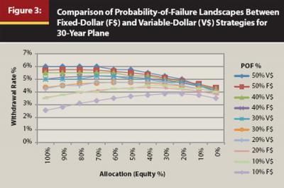
Figure 3, illustrating a commonly researched period, is similar to Figure 2, but shows both a variable dollar (V$) amount (spending retrenchment/expansion) strategy (Step 2) and the fixed-dollar (F$) strategy (Step 1) in order to illustrate the differences in withdrawal rate at the same probability of failure (POF). Notice that the variable-dollar probability-of-failure landscapes shift up; that is, the corresponding variable-dollar withdrawal rate is higher for each probability-of-failure landscape (Blanchett and Frank 2009). For example, at a 10 percent probability of failure, a 60 percent equity allocation results in a fixed 3.5 percent withdrawal rate, and the variable-dollar withdrawal rate is 4.2 percent.

When there is a difference along all time periods between comparative data sets, this suggests a possible strategy application (the greater the differences, the more effective the strategy and vice versa). The left side of Figure 4 represents a negative, or bad, market sequence for 35-, 25-, and 10-year periods for a strategy of withdrawal dollar amount adjustment (V$). The right side of Figure 4 represents a positive, or good, market sequence for the given period.

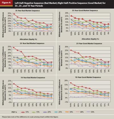
The differences in Figure 4 represent the percentage magnitude of change between the fixed-dollar withdrawals data (F$) in Step 1 and variable-dollar withdrawals data (V$) in Step 2 (as illustrated in Figure 3). For example, a 1 percent withdrawal rate change from 4 percent to 5 percent for a rising withdrawal rate (bad market, left side: portfolio value declines; hence, withdrawal rate increases) would represent a 25 percent change ((V$ – F$)/F$). Or a 20 percent change for the 1 percent withdrawal rate change from 5 percent to 4 percent for a declining withdrawal rate (good market, right side: portfolio value increases; hence, withdrawal rate decreases, (|(F$ – V$)/V$|). Absolute value is used here so that the magnitudes of change can be compared side by side in Figure 4. The comparison is between similar landscapes, for example 10%F$ to 10%V$ and so on.

The purpose of this strategy comparison is to see where probability-of-failure landscapes emerge as a decision point. Notice in Figure 4 that the differences between both strategy data sets compress and move closer to zero as the probability of failure increases; for example, the 50 percent POF percent data set differences are smaller than the 10 percent data set differences. This compression becomes more pronounced from 30 percent to 50 percent POF.

The compression of the withdrawal rate curves in Figure 4, or reduced differences between data sets (which means dollar adjustments are not as effective at this point), suggests that the withdrawal dollars should be adjusted as the probability of failure approaches 30 percent (probability of failure not to be confused with withdrawal rate), because this is when the compression of data differences begin to occur. Thus, results here suggest that a probability-of-failure range is a more useful approach. Of course, practitioners and their clients are free, indeed encouraged, to adopt lower probability-of-failure thresholds, for example, 20 percent, for the upper-range decision value.

The withdrawal rate differences are not consistent as the distribution period shortens; for example, for the bad market, 60 percent equity at 35 years, the data difference is 18.1 percent, but it is 7.9 percent at 10 years (both on the 15 percent probability-of-failure landscape).

Why 30 percent probability of failure as a maximum decision point? For probability-of-failure rates higher than 30 percent, differences in withdrawal rate data are much smaller, more sensitive to portfolio value changes, regardless of allocation. Thus more withdrawal dollar amount adjustments would be necessary to change probability-of-failure exposure; that is, at high probability of failure, risk changes quickly. The results in Figure 4 show that the amount of withdrawal rate change is not a constant, but changes depending on distribution period, portfolio allocation, and the probability of failure with which the retiree is comfortable.

Waiting for markets to improve the portfolio value later in order to improve the probability of failure (depending on the historical improvement of markets) may not be prudent because market improvements may be long in coming. The methodology developed here measures the probability of failure in order to prudently adjust the withdrawal rate sooner rather than later in response to what is actually occurring. Monitoring the improvement of probability of failure during moments of positive sequence risk provides a signal to increase the withdrawal dollar amount as well.

Practitioners should think in terms of returning their clients to within an acceptable range of probability of failure in both good and bad markets. The acceptable range for probability of failure should be client-specific per his risk tolerance. However, the higher the probability of failure (hence, withdrawal rate) the greater the necessary vigilance because it takes less of a portfolio value change to move quickly into even higher probability-of-failure rates (Figure 4). Readers are reminded to think in terms of an acceptable range of probability of failure because probability of failure will fluctuate as portfolio values fluctuate. Maintaining a fixed probability of failure is only possible by maintaining a fixed withdrawal rate, which translates to variable income when most retirees prefer a steady income (fewer retrenchments).

Step 3. Comparison of POF Landscapes Between Variable Portfolio Allocation (VA) Within Simulations and Fixed-Dollar (F$)

Garrison, Sera, and Cribbs (2010) dynamically change portfolio allocation during simulations using a trailing 12-month simple moving average as the portfolio-switching signal. Here we use the change in the portfolio value itself as the signal to switch between portfolios as described in methodology above. The results from this step will be compared with the fixed-dollar results from Step 1.

Figure 5 illustrates the withdrawal rate differences and compares fixed-dollar data (Step 1) to variable-allocation data (Step 3) between comparable probability-of-failure landscapes during either negative sequence (bad markets, left side) or positive sequence (good markets, right side). Percentage changes in the withdrawal rate are calculated the same here as in Figure 4.

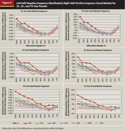
In Figure 5, the tolerable change of the withdrawal rate (the withdrawal amount compared with the portfolio value) is around 1 percent or less for bad market sequences. The probability-of-failure data differences are so small (values less than 1 in most cases) during bad market sequences that in this case a portfolio adjustment strategy would not enhance the retiree’s probability of failure.

The right side of Figure 5 represents a positive (good) market sequence for the stated distribution period. The percent change in withdrawal rate is much larger, comparable to that of increasing the withdrawal dollar amount in Step 2. However, that effect tends to disappear as the equity allocation is reduced to approximately 50 percent or less.

Changing portfolio allocation in response to sequence risk is ineffective in changing the probability of failure. The negative sequence (bad) market series (left side of Figure 5), has values so small, or even negative (indicating the fixed strategy has higher withdrawal rates), that they are essentially the same as the fixed-rate withdrawal rate values. Although the change in withdrawal rate values is large for the positive sequence (good) market series (right side of Figure 5), the dilemma is that this would imply allocating more aggressively during growing markets to take advantage of opportunities to increase the portfolio values but not allocating more conservatively during declining markets, which is not a practical or logical combination strategy.

These results suggest that changing portfolio allocation may be a more effective behavioral management tool. However, changing allocation solely to manage exposure to sequence risk and reduce exposure to probability of failure is not as effective as retrenchment. The general flatness of the withdrawal rate curves in Figures 2 and 3 also suggests this ineffectiveness because the withdrawal rates across the allocation spectrum are very close in value.

Further research combining a different allocation switching rule, for example one used by Garrison, Sera, and Cribbs (2010), with this probability-of-failure-based methodology would be interesting. Subsequent research is needed on integrating model-based rules with retiree behaviors during both adverse and positive sequence-risk periods.

Practical Applications

A retiree’s withdrawal rate, in reality, is not fixed. Recall that the withdrawal rate is a function of the withdrawal dollar amount divided by the portfolio value (with an inverse relationship to the market sequence): as market values go down, withdrawal rates go up and vice versa. Thus, over time, the withdrawal rate changes as a result of market effects on the portfolio value. The fundamental question is: at what withdrawal rate should a retiree be concerned during poor markets? Or, during good markets: how much more can the retiree afford to spend for a vacation?

However, as demonstrated above, using the withdrawal rate alone as the primary factor to answer these questions is problematic because the withdrawal rate depends on the retiree’s age (distribution time remaining). This paper shows that probability of failure automatically accounts for the withdrawal rate that corresponds to the remaining distribution period for each retiree. Thus, probability of failure forms the basis for adjusting the withdrawal amount. With his withdrawal dollar amount, a retiree transitions through various transient states as the markets change his portfolio values; that is, he transitions through probability-of-failure landscapes in Figure 1 as his portfolio values change.

For example, a retiree with a 20-year horizon and 60 percent equity allocation in a $1 million portfolio may currently have a 4.75 percent withdrawal rate that provides $47,500 annually with a 10 percent probability of failure (transient state 1). Shortly after, a poor market sequence may reduce the portfolio value to $913,462 for a withdrawal rate of 5.2 percent (transient state 2 with $47,500) at a 15 percent probability of failure. Continued poor markets may reduce the portfolio value to $772,358 for a 6.15 percent withdrawal rate with a corresponding 30 percent probability of failure (transient state n with $47,500). See Figure 2.

Therefore, the practical application comes from the ability to pre-calculate the corresponding portfolio values by using the withdrawal rates that correspond to various probabilities of failures, and have a discussion with the retiree beforehand about what his portfolio value thresholds may be for spending retrenchment decisions as well as providing time to make those spending changes as needed. Thus, this retiree needs to consider reducing expenditures to $36,687 (4.75 percent withdrawal rate of $772,358 to return back to the 10 percent probability-of-failure landscape) if he chooses to wait to make this decision at 30 percent probability of failure. Note that it is not certain the portfolio value will reach $772,358; however, should it do so, spending retrenchment is suggested at this point.

Most retirees would probably choose to retrench sooner, at a lower probability of failure, in order to have a higher distribution amount. However, prior to this paper, it was not clear at what point that retrenchment decision should be made. These portfolio values would be different for an older retiree who may have an 8 percent withdrawal rate (10-year distribution period), or a younger retiree who would have lower withdrawal amounts (30 years); however, the range of probability of failure up to a maximum value is useful in predetermining portfolio values for decisions for all retirees.

Because this is a dynamic process: a retiree who retrenches (or increases) spending needs to recalculate a new set of retrenched (or increased) portfolio values that represent his adjusted transient state rather than his prior state. That is, when his withdrawal dollar amount changes, the prior set of calculations no longer applies (for example, recalculating decision portfolio values based on $36,687 in the example above).

Notice that the authors are not suggesting either a 0 percent probability of failure or 30 percent probability of failure as absolutes. Rather, the suggestion is that portfolio values float as a result of market forces and thus a practical range of acceptable probability of failure needs to be recognized (otherwise, the retiree is constantly adjusting his withdrawal dollar amounts to maintain any given probability-of-failure landscape (Figure 1)). A range of probability-of-failure values generates a range of useful portfolio values with which a retiree can make more informed decisions beforehand.

The opposite applies for good market sequences. In the above example, the retiree may consider returning to his higher spending level as markets improve his portfolio value. For example, the retiree now has $1.2 million, and a 4.75 percent withdrawal rate (10 percent probability of failure) provides $57,000 this year; thus the retiree may consider using the $9,500 ($57,000–$47,500) for his vacation this year (with the understanding that poor market sequences may require future retrenchments).

Conclusion

The objective of our research is to establish probability-of-failure-based decision rules to aid practitioners in a forward-looking evaluation of retirees’ current exposure to sequence risk and to pre-determine portfolio values that may trigger retrenchment.

This paper introduces a method to demonstrate the concepts for purposes of broadening the perspective on sustainable distributions into three dimensions. The authors introduce the methodology to compare data sets of a proposed strategy against the baseline fixed-rate data to determine the efficacy of the proposed strategy and to determine refinements and possible break points for decisions using the proposed strategy.

A desire for low probability of failure comes with the cost of a low withdrawal rate requiring more assets to sustain distributions. However, the desire for a higher withdrawal rate (and therefore higher probability of failure) has the cost of increased sensitivity to sequence risk, resulting in more frequent dollar distribution adjustments to reduce probability of ruin. For these reasons, the authors suggest as more practical a range of retiree-acceptable probabilities of failure because portfolio values, which are what trigger the need for a decision, fluctuate—as opposed to control of the distributions to some specific probability-of-failure value, which implies a fixed withdrawal rate and thus variable withdrawal dollar amounts. In other words, either the withdrawal rate or the withdrawal dollar amount needs to fluctuate.

• Rather than a single safe withdrawal rate, there exists a range of withdrawal rates corresponding to varying degrees of probability-of-failure exposure.
• A higher relative probability of failure is more sensitive to a change in the current withdrawal rate (portfolio value); that is, even small changes in portfolio value (withdrawal rate) necessitate changes in dollar withdrawals, or retirees risk radical changes in probability of failure.
• The natural tendency would be to seek an optimal solution. Rather, an upper limit combined with a range of acceptable probability-of-failure values is more realistic because a transient-states perspective suggests fluidity.
• Changing the withdrawal amount is more effective in managing retiree exposure to sequence risk than changing the portfolio allocation.

In summary, the probability-of-failure results of each simulation, from a given set of distribution parameters, is a description of a single state that can be plotted three-dimensionally relative to other simulation probability-of-failure results that describe other sets of distribution parameters (Figure 1). The entire set of three-dimensional plots describes the distribution system. Each retiree moves through various states in a transient fashion as time and portfolio values change. Retiree actions, for example changing withdrawal amount or portfolio allocation, also change the transient state by changing the retiree’s probability of failure. Frank and Blanchett (2010) argue that exposure to sequence risk never goes away. This paper develops a methodology to evaluate that exposure to sequence risk for any given transient state and what retiree action may effectively change that sequence-risk exposure.

Endnote

1. An extended version of this research working paper is available at SSRN: http://ssrn.com/abstract=1849868.

References

Blanchett, David M., and Larry R. Frank. 2009. “A Dynamic and Adaptive Approach to Distribution Planning and Monitoring.” Journal of Financial Planning 22, 4: 52–66.

Frank, Larry R., and David M. Blanchett. 2010. “The Dynamic Implications of Sequence Risk on a Distribution Portfolio.” Journal of Financial Planning 23, 6: 52–61.

Garrison, Michael M., Carlos M. Sera, and Jeffrey G. Cribbs. 2010. “A Simple Dynamic Strategy for Portfolios Taking Withdrawals: Using a 12-Month Simple Moving Average.” Journal of Financial Planning 23, 2: 51–61.

Guyton, Jonathan T. 2004. “Decision Rules and Portfolio Management for Retirees: Is the ‘Safe’ Initial Withdrawal Rate Too Safe?” Journal of Financial Planning 17, 10: 54–62.

Guyton, Jonathan T., and William J. Klinger. 2006. “Decision Rules and Maximum Initial Withdrawal Rates.” Journal of Financial Planning 19, 3: 49–57.

Mandelbrot, Benoit, and Richard L. Hudson. 2004. The Misbehavior of Markets: A Fractal View of Financial Turbulence. New York: Basic Books.

Mitchell, John B. 2011. “Withdrawal Rate Strategies for Retirement Portfolios: Preventive Reductions and Risk Management.” Financial Services Review (forthcoming). An earlier version is available at: http://ssrn.com/abstract=1489657

Pye, Gordon B. 2008. “When Should Retirees Retrench? Later Than You Think.” Journal of Financial Planning 21, 9: 50–59.

Stout, R. G. 2008. “Stochastic Optimization of Retirement Portfolio Asset Allocations and Withdrawals.” Financial Services Review 17: 1–15.

Taleb, Nassim N. 2007. The Black Swan: The Impact of the Highly Improbable. New York: Random House.