Understanding the Intersection Between Style Exposure, Sector Rotation, and the Business Cycle

Journal of Financial Planning: May 2021

 

Executive Summary

• Financial planners and investors generally tend to evaluate their equity allocation either through the lens of sector exposure or through the lens of style exposure. In reality, these two dimensions are highly related.
• Using holdings-based style analysis, this research shows that the average funds in the Morningstar large-cap growth and large-cap value categories tend to overweight or underweight certain sectors relative to the broad stock market, while SPDR sector ETFs vary greatly in their exposure to growth and value stocks.
• Returns-based style analysis based on the Fama-French Three-Factor Model confirms that certain sectors exhibit strong and consistent style biases. Specifically, the technology sector has historically exhibited the strongest growth bias, while the financial sector exhibited the strongest value bias.
• After introducing a relatively simple definition of the business cycle, authors proceed to analyze the performance of sectors through the different phases of the cycle and demonstrate that certain groups of sectors tend to consistently perform better in specific phases of the cycle.
• Authors demonstrate how a relatively simple investment strategy that actively rotates between sectors—based on changes in the business cycle—would have consistently and significantly outperformed the broad stock market. Authors then analyze the style characteristics of such a strategy.
• This paper concludes by showing that the aforementioned strategy, when implemented as a 15 percent satellite to an otherwise passive and broadly diversified portfolio, would significantly improve the risk/return characteristics of the portfolio.

 

Carl Noble, CFA, is the senior vice president of investments at Congress Wealth Management, LLC. Previously, he was chief investment officer of Pinnacle Advisory Group, Inc.

Sean Dillon, CMT, CFTe, is the senior vice president of investment strategy at Congress Wealth Management, LLC. Prior to that, he was the chief investment strategist for Pinnacle Advisory Group, Inc. He holds the Series 65 certification.

Sauro Locatelli, CFA, FRM, SCR™, is the director of quantitative research for Congress Wealth Management, LLC. Prior to that, he held the same position at Pinnacle Advisory Group, Inc. 

 Dan Mento, CFA, is a portfolio manager. Formerly, he was he fixed income analyst at Pinnacle Advisory Group, Inc. He also worked at T. Rowe Price and Bank of New York Mellon. 

Ken Solow, CFP^®, is a founder of Pinnacle Advisory Group, Inc.  He is the author of the book, Buy and Hold is Dead Again: The Case for Active Management in Dangerous Markets.

JOIN THE DISCUSSION: Discuss this article with fellow FPA Members through FPA's Knowledge Circles. ​​

FEEDBACK: If you have any questions or comments on this article, please contact the editor HERE. 

NOTE: Please click on images below to open PDF versions.

Financial planners and investors generally tend to evaluate their equity allocation either through the lens of sector exposure or through the lens of style exposure. In reality, these two dimensions are highly related.

Using holdings-based style analysis, this paper shows that the average funds in the Morningstar large-cap growth and large-cap value categories tend to overweight or underweight certain sectors relative to the broad stock market, while SPDR sector ETFs vary greatly in their exposure to growth and value stocks. This paper also demonstrates how a relatively simple investment strategy that actively rotates between sectors based on changes in the business cycle would have consistently and significantly outperformed the broad stock market, and analyzes the style characteristics of such a strategy.

Literature Review

Two major approaches to portfolio construction, as well as two major dimensions along which a portfolio’s exposure can be deconstructed and analyzed, are asset allocation and style or factor allocation. Vardharaj and Fabozzi (2007) found that nearly three-quarters of the cross-sectional variation of five-year returns of U.S. funds can be explained by either sector or style allocation policy. While an extensive body of research has been dedicated to each of these two dimensions individually, research on how the two approaches interact with each other has been more limited. Idzorek and Kowara (2013) compared a factor-based approach to asset allocation and an asset-class-based approach to asset allocation and concluded that neither one is inherently superior. Their results suggested that both approaches should be taken into account by investors.

Angelidis and Tessaromatis (2017) exposed how the asset allocation and style selection interact with each other within the context of country allocation. They proposed an alternative to stock-based factor portfolios by constructing country-based factor portfolios using country ETFs or index futures. Their research concluded that such country-based factor portfolios would be able to effectively capture the premium associated with factors such as small capitalization and value, while being cheaper to trade due to greater liquidity. Finally, a notable attempt to combine the two approaches was made by Bender, Le Sun, and Thomas (2018). They proposed a methodology for integrating factor allocation and asset class return prediction in a way that allows information/forecasts of factors and asset classes to be used in conjunction, resulting in optimal portfolios that blend insights from both paradigms.

This research seeks to build on the existing literature by focusing on how asset allocation and style selection interact within the context of U.S. equity sectors.

Exploring Style Analysis Through the Lens of  U.S. Equity Sectors

The investment style of mutual fund managers and separate account managers is often determined by their approach to using S&P 500 sectors and industries as a basis for individual stock selection. “Top-down” fund managers actively “rotate” their ownership of U.S. stocks among equity sectors based on their evaluation of the market and economic cycle.

Alternatively, “bottom-up” fund managers often utilize stock screens based on a variety of factors, including (but not limited to) size, growth/value, momentum, quality, and volatility, which result in buying stocks that fit those criteria, regardless of which sector they belong to.

The outcome of either “bottom-up” or “top-down” stock selection result in portfolio style characteristics that are typically set forth in the fund prospectus. Hence, the fund managers’ stock selection criteria result in a mutual fund being classified as a growth or value fund and is often marketed as such by the fund distributor. Financial planners then use either holdings-based style analysis or performance-based style analysis to make their own assessment of an active manager’s investment style.

This paper analyzes 11 different U.S. equity sectors using Morningstar’s holdings-based style box methodology. Authors then use the Fama-French Three-Factor Model to evaluate GICS sectors’ growth and value characteristics using a performance-based style methodology. The paper concludes by offering a strategy for actively and tactically managing U.S. equity sectors using a “top-down” approach to opportunistically earn excess returns as sector performance changes during the evolution of a typical economic cycle, and analyzing the style characteristics of such a strategy.

About S&P 500 GICS Sectors

In 1999, MSCI and S&P Dow Jones developed the Global Industry Classification Standard (GICS). GICS uses a four-tiered system with both quantitative and qualitative inputs to assign each company in the S&P 500 Index a single sub-industry classification according to its principal business activity.¹ Currently, the S&P 500 Index is divided into 11 different sectors, 24 industry groups, 69 industries, and 158 subindustries according to this system. The classifications are reviewed annually and have been revised many times since being created.

For the purposes of this paper, the focus will be on these 11 sectors: communication services, consumer discretionary, consumer staples, energy, financials, healthcare, industrials, information technology, materials, real estate, and utilities. For investors, these are directly accessible through mutual funds and exchange-traded funds (ETFs) that closely track the sector indices. Fidelity helped pioneer sector investing—creating the first sector mutual fund in 1981—while sector-based ETFs first became available in 1998.

This research begins by looking at the sector weightings of mutual funds in the Morningstar Large-Cap Value and Large-Cap Growth categories using holdings-based style analysis provided by Morningstar’s style-box methodology.²

As can be seen in the left panel of Table 1, Morningstar’s methodology for determining growth and value characteristics results in the value style box including funds with the largest differential GICS sector weightings in financials, energy, utilities, and staples—and the growth style box including funds with the largest differential weightings in technology, consumer discretionary, communication services, and healthcare.

 

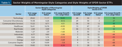
Next, authors analyze each of the S&P 500 GICS sectors to see how Morningstar categorizes the stocks owned in each individual sector SPDR ETF. The results are shown in the right panel of Table 1.

According to Morningstar, the stocks in the technology sector ETF can be broken down to 48 percent large growth, 34 percent large blend, and 12 percent large value, which is consistent with the composite of the large-cap growth style box where technology stocks represented 29.62 percent of the holdings, versus only 11.17 percent of the large-cap value style box. This approach seems to confirm the value and growth characteristics of individual GICS sectors, with technology, communication services, and consumer discretionary stocks being significantly tilted to growth, and financial, energy, staples, and utilities stocks being significantly tilted toward value.

The one discrepancy worth noting is healthcare, where the holdings of healthcare stocks in the large-growth style box is roughly equal to the healthcare stocks in the large-value style box, (16.41 percent versus 16.76 percent, respectively), but when analyzing the GICS SPDR Healthcare Sector ETF, the allocation tilts toward blend and value where the weights are 13 percent large growth, 47 percent large blend, and 31 percent large value. It is notable that when evaluating each individual GICS sector SPDR ETF there is a mix of value, blend, and growth stocks. Investors do not appear to get a “pure” exposure to any one investment style when focusing on sector investing using a holdings-based approach.

Applying the Fama-French Three-Factor Model to S&P 500 GICS Sectors

While style investing using mutual funds and sector investing using ETFs tend to be viewed as different and unrelated approaches to investing, the truth is they are strongly connected to each other.

As shown above, different sectors have clear and distinct style characteristics, with certain sectors having a significantly larger exposure to value (e.g., financials) and other sectors having a significantly larger exposure to growth (e.g., technology). This paper has shown that when using Morningstar’s methodology for determining value and growth, style-based portfolios tend to consistently overweight or underweight certain sectors relative to a broad market index.

As an alternative to using the Morningstar style methodology, we can demonstrate that sectors have style biases by applying the Fama-French Three-Factor Model to the eleven sectors of the S&P 500 index, using a dataset of monthly returns from 1990 to 2020. As opposed to the Morningstar Style Box, which is a form of holdings-based style analysis, the Fama-French Three-Factor Model is a form of returns-based style analysis. This means that the style characteristics of a given fund are estimated based solely on the fund’s performance over a given time frame through the use of regression analysis, with no regard for the fundamentals of the underlying stocks.

In 1965, Eugene Fama published his hypothesis known as the Capital Asset Pricing Model that identified risk premium in the market based on a security’s beta, or market risk. This was later expanded upon in 1992 with the help of Kenneth French in the creation of the Fama-French Three-Factor Model to include size and value along with risk premium (Fama and French 1992). 

This research starts by regressing monthly sector returns against the Fama-French three factors over the full length of the sample. The results of these regressions show that on the average style characteristics of each sector over the whole period. In addition, this paper also applies the Fama-French Three-Factor Model to the broad S&P 500 index as well as to the S&P 500 Value index and the S&P 500 Growth index.³

The left panel of Table 2 reports all three coefficients, plus the alpha component or intercept, resulting from the Fama-French Three-Factor Model. The fourth column of the table contains the “High Minus Low” (HML) coefficient for each sector. The HML coefficients measure each sector’s sensitivity to the value premium, with a higher coefficient indicating a higher exposure to value and a lower coefficient indicating a higher exposure to growth. The sectors in the table have been ranked by HML coefficient, from highest to lowest.

 

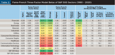
Based on the results shown in the left panel of Table 2, the following observations can be made:

• The S&P 500 index has an HML coefficient of 0.04, which is statistically indistinguishable from zero. Eight out of the 11 sectors of the S&P 500 have a HML coefficient that is positive and greater than that of the S&P 500 index as a whole, while only three sectors have a negative HML coefficient.
• The HML coefficient can vary significantly across sectors. The sector with the highest HML coefficient is financials (0.71), while the sector with the lowest HML coefficient is technology (–0.65). The spread in HML coefficient between these two sectors equals 1.35. That is more than twice as large as the spread in HML coefficient between the S&P 500 Value index and the S&P 500 Growth index, which is equal to 0.58.
• Four sectors have a HML coefficient greater than that of the S&P 500 Value index (0.34). These sectors are financials (0.71), energy (0.51), real estate (0.50), and materials (0.41). One sector has a HML coefficient that is smaller than that of the S&P 500 Growth index (–0.24), and that sector is technology (–0.65). Investing in these sectors directly may be a way for investors to achieve greater exposure to value or growth than that offered by investments tracking the S&P 500 style indexes.

These results are consistent with the average sector weights of the Morningstar Large Cap Value and Large Cap Growth, shown previously in Table 1.

Authors estimated the average style characteristics of the sectors over the entire sample. However, it hasn’t yet been determined how consistent and reliable these style characteristics are over time. In other words, authors have determined that the financial sector, on average, tends to have a high sensitivity to value—but does it consistently behave that way or are there times when the sector behaves more like growth?

In order to answer this question, authors subdivide the database of 371 monthly returns into a set of 336 partially overlapping 36-month periods, with the first 36-month period starting Dec. 31, 1989, and ending Dec. 31, 1992, and the last 36-month period starting Nov. 30, 2017, and ending Nov. 30, 2020. A period length of 36 months (i.e., 36 observations) is generally considered to be long enough to provide statistically valid results, while being short enough to provide a snapshot of a given point in time (Mason, McGroarty, and Thomas 2012). The Fama-French Three-Factor Model is then applied to each of these 36-month periods, obtaining a set of coefficients (and specific to our purpose, a HML coefficient) for each of these periods. Authors can then determine the consistency and reliability of a given sector’s style characteristics by observing the variability of its 36-month HML coefficient over time. The results of these regressions are shown in the middle panel of Table 2.

In looking at the average 36-month HML coefficients of the 11 sectors, one can see that they are generally consistent with the HML coefficients for the entire sample period. Specifically:

• Seven sectors have positive average 36-month HML coefficient, while four sectors have negative average 36-month HML coefficient.
• Financials is the sector with the highest average 36-month HML coefficient (0.68), while technology is the sector with the lowest average 36-month HML coefficient (–0.66).
• Other sectors also follow a similar distribution as in the prior table: energy, materials, utilities, and real estate still exhibit a relatively high average 36-month HML coefficient, while healthcare, staples, and communication services exhibit a relatively low (and negative) average 36-month HML coefficient.

However, what authors are concerned with the most here is not the average 36-month HML coefficients, but their variability over time. The second and third columns in the middle panel of Table 2 show the highest and lowest 36-month HML coefficient for each sector during this study sample. The fourth column shows the spread between the two. These columns show that there is indeed a significant amount of variability in the style characteristics of sectors over time. This is not surprising, given that even the S&P 500 Value and S&P 500 Growth indexes exhibit some amount of variability in their 36-month HML coefficient.

The only sector that can be said to have always had a consistent style exposure during the entire sample is the financial sector, which had a highest and lowest 36-month HML coefficient of 1.360 and –0.03, respectively. While –0.03 is technically negative, it is close enough to zero to characterize it as being neither value nor growth. Therefore, while it cannot be said that the financial sector has always behaved like value, it can be said that it has never really behaved like growth.

The financial sector also exhibited one of the lowest spreads between the highest and lowest 36-month HML coefficients, at 1.39. With most other sectors, there was greater variability in 36-month HML coefficients, with many sectors having, at times, exhibited strong value tendencies—and at other times exhibited similarly strong growth tendencies. Worthy of special notice is the energy sector, which appears to have exhibited the greatest variability in its 36-month HML coefficient, with a 3.09 spread between the highest and lowest 36-month HML coefficients. In fact, the energy sector’s highest 36-month HML coefficient of 2.12 is considerably higher than that of the financial sector (1.36). However, the energy sector’s lowest 36-month HML coefficient of –0.97 was the third lowest of all the sectors, after technology’s –1.60 and healthcare’s –1.31.

An alternative way to gauge the reliability of a given sector’s style characteristics is to rank the 11 sectors’ 36-month HML coefficients from highest to lowest at each point in time in this sample, and to look at how often a given sector appears near the top of the ranking as opposed to near the bottom of the ranking. The right panel of Table 2 summarizes the results of this exercise. The three leftmost columns report the average rank of each sector throughout the sample, as well as the sector’s highest and lowest rank. The two rightmost columns report the percentage of time that each sector was ranked among the top three and the bottom three sectors based on their 36-month HML coefficient.

Based on these results, the following observations can be made:

• The financial sector has the highest average rank, while the technology sector has the lowest average rank. This is consistent with the results shown in prior tables.
• From the highest rank columns, notice that seven different sectors held the No. 1 ranking at different points in time. Moreover, from the lowest rank column, notice that six different sectors held the No. 11 ranking at different points in time. In other words, there is quite a bit of variability in the ranking over time.

That being said, some of the sectors do display a relatively consistent style signature over time.

• The financial sector’s 36-month HML coefficient was ranked among the top three sectors 81.7 percent of the time, and was ranked among the bottom three sectors only 1.2 percent of the time.
• The technology sector’s 36-month HML coefficient was ranked amount the bottom three sectors 81.4 percent of the time, and was only ranked among the top three sectors 4.6 percent of the time.
• The healthcare sector’s 36-month HML coefficient was ranked among the bottom three sectors 69.8 percent of the time and was ranked among the top three sectors only 1.2 percent of the time.
• Other sectors appeared both among the top three and the bottom three sectors ranked by 36-month HML coefficient, but some of them appeared much more frequently at the top of the ranking than at the bottom (e.g., energy, materials), while others appeared much more frequently at the bottom of the ranking than at the top (e.g., consumer staples, communication services)

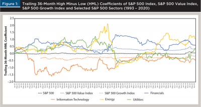
Finally, Figure 1 shows a visual representation of how the 36-month HML coefficient can vary over time. The S&P 500 growth and value indices are constructed to always provide exposure to growth and value, respectively. However, as Figure 1 shows, even their 36-month HML coefficient is subject to a certain degree of variability. Moreover, observe that some sectors, such as financials and technology, tend to consistently behave as value and growth, respectively. Other sectors, such as energy and utilities, have shifted from value to growth and vice versa.

 

Sector Rotation Through the Business Cycle

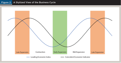
In order to understand how sector performance changes as the economy moves through its different phases, business cycle must first be defined. In order to do this, both the Leading Economic Index (LEI) and the Coincident Economic Indicators (CEI), as published by the Conference Board, are used.⁴        

The LEI consists of 10 different economic indicators that tend to lead turning points in the U.S. economy, while the CEI consists of four different indicators that tend to change at approximately the same time as the economy. Both have extensive histories dating back to the late 1950s, covering several business cycles.

By combining the two, authors can clearly delineate the distinct phases of the business cycle, as shown in a stylized way in Figure 2: an economic contraction is the period from the peak in the CEI to an ensuing trough in the LEI; an early economic expansion is the period from the trough in the LEI to the trough in the CEI; a mid-economic expansion is the period from the trough in the CEI to the peak in the LEI; and a late economic expansion is the period from the peak in the LEI to the peak in the CEI. At the expense of excluding other factors that affect the business cycle, this relatively simplistic definition allows us to objectively and quantitatively mark the turns in the cycle.

 

From there, historical returns can be examined to illustrate how sector performance is influenced by changes in the economy. Table 3 shows the average monthly relative performance for the 11 sectors of the market using data from 1972 to 2020.

 

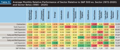
The relative performance is calculated by taking the difference between the sector’s return and the overall return for the S&P 500 Index excluding the sector. On the right-hand side of Table 3, we have simplified the analysis by aggregating sectors into three main groups: early cycle sectors, late cycle sector, and defensive sectors.

The early cycle sectors are consumer discretionary, financials, and technology. As a group, they tend to outperform in the early phase of economic expansions after interest rates have been lowered and there is still plenty of slack in the economy.

The late cycle sectors are energy, industrials, and materials, which tend to outperform as an economic expansion ages and inflation begins to rise as economic slack dissipates. The defensive sectors are communication services, consumer staples, healthcare, and real estate, which tend to outperform as the economy slides into a new contraction, mainly due to the consistency and stability of earnings for the companies in these sectors, which allows them to better withstand economic weakness.⁵ This is also borne out by comparing historical sector betas versus the S&P 500 Index.

As shown at the bottom of Table 3, on average, the early cycle sectors have a beta greater than 1 (i.e., the beta of the market), the late cycle sectors have a beta of approximately 1, and the defensive sectors carry a beta that is lower than 1. This is further supported by historical sector performance shown in Table 3, which shows that early cycle sectors have performed best during the early expansion phase of the economic cycle, late cycle sectors have performed best during the late expansion phase, and the defensive sectors have performed best in the contraction phase.

The Benefits and Style Implications of Sector Rotation Through the Business Cycle

This section will illustrate the potential benefits that could be reaped by changing the composition of a hypothetical portfolio during the different phases of the business cycle, as defined in the prior section. An example of prior research on the subject is offered by Chong and Phillips (2015), who implemented a strategy that attempted to outperform the broad market by alternating between sectors during different stages of the business cycle, based on a set of 18 economic factors. They concluded that there is the potential for such strategies to outperform the broad market—even rebalancing the portfolio as infrequently as twice per year. This research assumes that its hypothetical portfolio will be managed as follows:

• During the early and middle stages of the business cycle, 100 percent of the portfolio will be invested in early cycle sectors (consumer discretionary, financials, technology), weighted according to their respective weights in the S&P 500.
• During the late stage of the business cycle, 100 percent of the portfolio will be invested in late cycle sectors (energy, industrials, materials), weighted according to their respective weights in the S&P 500.
• During contractions in the business cycle, 100 percent of the portfolio will be invested in defensive sectors (staples, healthcare, utilities, real estate, telecommunication), weighted according to their respective weights in the S&P 500.

As a reminder, we are defining the different phases of the business cycle through the intersection of the CEI and LEI, which are published by the Conference Board every month. As such, the strategy could be replicated in real time, without the benefit of hindsight.

From February 1990 to November 2020, the sector rotation portfolio would have achieved an annualized return of 14.40 percent, compared to just 10.40 percent for the S&P 500 index, its natural benchmark. Just to give an idea of how such a large difference in annualized return would compound over time, $1 million invested in the sector rotation portfolio in 1990 would have grown to $63.38 million in 2020, while a similar investment in the passive benchmark would have grown to just $21.11 million.

The sector rotation portfolio would have been somewhat riskier than the passive benchmark, as indicated by its higher standard deviation of 16.81 percent, compared to 14.66 percent for the benchmark, as well as by its beta of 1.05 relative to the S&P 500 index. However, such high beta was not the primary source of outperformance, as the sector rotation portfolio would have outperformed its benchmark, even on a risk-adjusted basis.

The portfolio’s Sharpe ratio of 0.70 would have been significantly higher than the benchmark’s Sharpe ratio of 0.53, and the portfolio would have delivered an annualized alpha of 3.62 percent. The standard deviation of the monthly alpha would have been 6.94 percent, resulting in an information ratio of 0.52. These numbers are evidence that a significant portion of the portfolio’s outperformance would have resulted not from its higher risk, but from selecting the most favorable sectors for each phase of the business cycle.

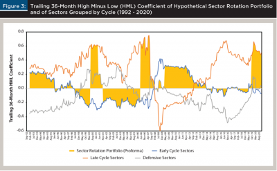
Next, this paper turns its attention to the style characteristics of such a sector rotation portfolio and analyzes how they would have evolved through the business cycle. Figure 3 plots the trailing 36-month HML coefficient of the sector rotation portfolio from 1990 to 2020. Figure 3 also plots the trailing 36-month HML coefficient of early cycle sectors, late cycle sectors, and defensive sectors. In addition, Table 4 shows the average trailing 36-month HML coefficient of the portfolio during the different phases of the cycle.

 

 

 

Based on this information, the following observations can be made:

• During the early and middle phases of the cycle, by construction, the portfolio would be invested in early cyclical sectors. It is within this group of sectors that we find both the sector with the most significant value exposure (financials) and the sector with the most significant growth exposure (technology). As a result, the portfolio would exhibit a fairly neutral value/growth style exposure over time, with its trailing 36-month HML coefficient averaging 0.04 and rarely venturing outside of the –0.30 to 0.30 range.
• During the late stage of the cycle, the portfolio would be invested in late-cycle sectors: energy, industrials, materials. In this stage, the portfolio would clearly exhibit a large exposure to value, with a trailing 36-month HML coefficient averaging 0.55 and often reaching or exceeding 0.6.
• During contractions, the portfolio would be invested in defensive sectors. During this time, the portfolio would end up being tilted towards value, but to a much smaller extent compared to the late stage of the cycle. The average trailing 36-month HML coefficient of the portfolio during contractions was 0.15.

Finally, on Figure 3 it is worth noting the behavior of late cycle sectors during the late stages of the business cycle. While late-cycle sectors, on average (i.e., throughout the cycle) appear to have the most exposure to value, it is interesting to note that their value-like behavior is heightened during the late phase of the cycle, which is exactly when our hypothetical portfolio would be rotating toward these sectors. This highlights the importance for investors to be aware of the relationship between sector allocation and style exposure, as changing the portfolio composition alongside one of these two dimensions can heavily influence the other.

A Core and Satellite Approach

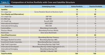
From the perspective of a financial planner, allocating the entirety of a client’s portfolio to only three or four U.S. Large Cap sectors at any point in time would be considered irresponsible due to a lack of diversification. However, this section demonstrates how such an investment strategy can be successfully implemented at a smaller scale within the context of a more diversified portfolio, using a core and satellite portfolio structure.

Consider two hypothetical, broadly diversified portfolios as described in Table 5. The only difference between the active portfolio and the passive portfolio is that the active portfolio features a 15 percent satellite that is invested in the hypothetical sector rotation strategy described in the prior section. The 15 percent allocation for the satellite was carved out from the passive allocation to U.S. Large Cap. As such, any differential in performance between the two portfolios can be attributed to the hypothetical sector rotation strategy’s performance relative to the S&P 500.

 

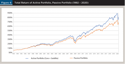
Between February 1993 and November 2020, the active portfolio would have produced an annualized return equal to 8.66 percent, compared to just 8.05 percent for the passive portfolio. Thus, the active portfolio would have outperformed by 0.61 percent per year. The active portfolio would have outperformed on a risk-adjusted basis as well. Its Sharpe ratio of 0.66 would have been greater than the passive portfolio’s 0.61. Moreover, the active portfolio would have delivered an annualized alpha of 0.52 percent, with a beta of 1.01. The standard deviation of monthly alpha would have been 1.03 percent, resulting in an information ratio equal to 0.50. Figure 4 plots the total return of the two portfolios. One million dollars invested in the active portfolio at the beginning of 1993 would have grown to a portfolio value of $10.1 million in November 2020, compared to just $8.6 million for the passive portfolio.

 

These results confirm that the hypothetical sector rotation strategy, even when confined to the satellite portion of the portfolio, can be a useful tool for financial planners in helping their clients achieve their goals. These performance numbers include the reinvestment of dividends but do not consider the impact of expense ratios, transaction costs, and taxes. Expense ratios would lower the returns of both portfolios by a similar magnitude and, therefore, are irrelevant when evaluating the relative performance between the two portfolios.

At the time of this writing, transaction costs at nearly every major U.S. stock brokerage and/or custodian have fallen to negligible levels and can be safely disregarded when considering the application of this strategy going forward. Regarding taxes, financial planners implementing such a strategy should take asset location into account and ensure that the sector rotation satellite, which is the least tax-efficient component of the portfolio, is located inside tax-sheltered accounts as much as possible. To the extent that the 15 percent satellite is fully located inside tax-sheltered accounts, then the tax implications of such a strategy can be safely disregarded.

Conclusion

This paper demonstrated that style analysis and sector rotation are intertwined. It also showed that as a financial planner constructs a portfolio using growth and value funds in each Morningstar style box, they are implicitly making choices about equity sectors as well.

This analysis used the Fama-French Three-Factor model to test GICS sectors for growth and value characteristics. The authors observed that over time, equity sectors have varying style characteristics. Some sectors have shown consistent exposures to value or growth styles, while others are more inconsistent, shifting between value and growth over time.

Understanding the style characteristics of sectors can help investors make informed decisions within the context of the business cycle. This paper showed that since 1972, early cyclicals like technology and consumer discretionary have performed best during the early and mid-expansion periods of the business cycle. Late cyclical sectors have historically performed their best during late expansionary periods. During periods of economic contraction, defensive sectors such as staples and healthcare have outperformed.

As a result of these sector and style relationships, style investors can benefit from an awareness of the underlying sectors they own. A sector rotation strategy based on the business cycle can consistently outperform the broad market on a return basis as well as on a risk-adjusted basis. When implementing such a strategy, investors would still be able to incorporate their style views in choosing which sectors to own. This research also showed that such a strategy can be successfully implemented within the context of a core and satellite portfolio structure, making it suitable for wealth management clients. This more nuanced approach to building portfolios should result in more robust strategies and better-informed investors.

Endnotes

1. See The Global Industry Classification Standard (GICS) at msci.com/gics.
2. Learn more about the Morningstar Style Box Methodology at morningstar.com/content/dam/marketing/shared/research/methodology/678263-StyleBoxMethodolgy.pdf.
3. See “S&P U.S. Style Indices Methodology” at spglobal.com/spdji/en/documents/methodologies/methodology-sp-us-style.pdf.
4. See the description of components from The Conference Board at conference-board.org/data/bci/index.cfm?id=2160.
5. See the paper from Massey University’s Department of Finance and Economics, “Sector Rotation over Business Cycles,” by Jeffrey Stangl, Ben Jacobsen, and Nuttawat Visaltanachoti at researchgate.net/profile/Ben_Jacobsen/publication/228425439_Sector_rotation_over_business-cycles/links/53db67ac0cf2631430cb4896.pdf.

References

Angelidis, Timotheos, and Nikolaos Tessaromatis. 2017. “Global Equity Country Allocation: An Application of Factor Investing.” Financial Analysts Journal 73 (4): 55–73.

Bender, Jennifer, Jerry Le Sun, and Ric Thomas. 2018. “Asset Allocation vs. Factor Allocation—Can We Build a Unified Method?” The Journal of Portfolio Management 45 (2): 9–22.

Chong, James, and G. Michael Phillips. 2015. “Sector Rotation with Macroeconomic Factors.” The Journal of Wealth Management 18 (1) 54–68.

Fama, Eugene F., and Kenneth R. French. 1992. “Common Risk Factors in the Returns of Stocks and Bonds.” Journal of Financial Economics 33 (1): 3–56.

Idzorek, Thomas M., and Maciej Kowara. 2013. “Factor-Based Asset Allocation vs. Asset-Class-Based Asset Allocation.” Financial Analysts Journal 69 (3): 19–29.

Mason, Andrew, Frank McGroarty, and Steve Thomas. 2012. “Style Analysis for Diversified U.S. Equity Funds.” Journal of Asset Management 13 (3): 170–185.

Vardharaj, Raman, and Frank J. Fabozzi. 2007. “Sector, Style, Region: Explaining Stock Allocation Performance.” Financial Analysts Journal 63 (3): 59–70.