Journal of Financial Planning: May 2018
Arthur Cox, Ph.D., is professor of finance and director of the Center for Real Estate Education in the Department of Finance at the University of Northern Iowa. His research interests include real estate valuation and finance, agency, and real estate development.
Richard Followill, Ph.D., is a professor of finance at the University of Northern Iowa. His research interests include real estate finance, real estate development, investments, and market efficiency. He has published numerous articles in peer-reviewed publications such as the Journal of Real Estate Research, The Appraisal Journal, and The Engineering Economist. In addition, he authored Spreadsheet Models for Investments.
Author’s note: An Excel spreadsheet of the methodology, data, and results produced for this study and referenced throughout this paper is available for download for free from the Center for Real Estate Education at the University of Northern Iowa at realestate.uni.edu/research-papers-articles-informative-writing#.
Executive Summary
- Past studies have suggested that home ownership is superior to renting, and a number of rent-versus-buy calculators exist; many of which support this finding.
- These calculators, however, often do not incorporate all the expenses involved with either homeownership or renting, and many assume a short time horizon despite the fact that many families maintain households for decades.
- This paper presents long-term, historical scenarios for six metropolitan areas that compare accumulated ending wealth for the rent-versus-buy decision. The scenarios incorporate the major costs of home ownership and renting over a 30-year time horizon.
- These historical scenarios, which reflect year-to-year changes in such factors as mortgage rates and investment returns, show that home ownership has not always been the best financial decision for a family.
Imagine a young family comes to you, their financial planner, with this question: “Are we better off to buy or rent a home?” What would be your response? Many financial planners would likely provide the answer that a lot of clients would expect: buy. Some previous studies acknowledge this response. Beracha and Johnson (2012) stated, “The concept of homeownership seems to be entrenched in our national psyche” (page 217). According to Di, Belsky, and Liu (2007), “Most people take it as an article of faith that owning a home is the best way to accumulate wealth” (page 275), and their research concluded that homeownership was positively and significantly associated with wealth accumulation over time. However, if “buy” is your answer to this young family’s question, how confident are you in that response? And on what basis do you offer it?
The purpose of this study is to provide background for this decision by analyzing whether families in six different metropolitan areas would have been better off financially had they rented or owned their home over the 30-year period between 1984 through 2013. This study showed that the consequences of this decision are not always in favor of home ownership.
The historical data presented suggests that the home ownership decision should not be uniformly adopted. This result is demonstrated by evaluating the rent-versus-buy decision using net ending wealth as the relevant criterion.
To provide context, however, issues in addition to ending wealth should be mentioned. Owning a home can provide financial stability that might not exist from renting. Financial stability could be enhanced through home ownership by less volatile fixed mortgage payments and from what may be considered forced savings as equity accumulates due to the paydown of the mortgage and appreciation of home value. In addition, many families have a pride of ownership that does not exist for renters. Renting, however, may mitigate the uncertainty arising from repairs and maintenance as these are commonly the responsibility of the landlord. Renting also facilitates mobility, for example, when changing jobs.
Literature Review
The rent-versus-buy decision has been considered by many authors in both the trade and popular press. An article on Realtor.com (Stults 2015) used the number of affordable homes in a market as the measure for determining whether it was better to rent or own. A maximum affordable price was estimated, and the properties available with a price below that level were deemed affordable. Others have used a home price-to-income ratio (Case and Shiller 2004; McCarthy and Peach 2004; Beracha and Hirschey 2009). A market is considered overvalued or undervalued based on this ratio, which can be used as the criterion for buying versus renting. Another method, used by Martin (2008), employed a ratio based on home ownership costs versus renting costs.
Another decision criterion, called the horse-race comparison, pits the total cost of owning versus that of renting. Beracha and Johnson (2012) used ending wealth as their decision criterion, and assumed home ownership was initially costlier than renting. Ending wealth from home ownership incorporated the selling price of the home. For the renter, ending wealth included the invested savings resulting from the lower cost of renting. Rent was inflated at an assumed constant rate, and the annual difference between renting and owning was either added to or subtracted from the amount available for investment for each year of rolling eight-year time horizons. The authors concluded that from a purely pecuniary perspective, a family would have been better off renting during much of the time between 1978 and 2009.
Smith and Smith (2004) used net present value of after-tax cash flows as their decision rule. They accounted for the expenses of home ownership as well as the tax savings resulting from the deductibility of interest and property taxes. The initial amount for rent was approximately equal to the mortgage payment. Except for the fixed-mortgage payment, housing expenses for both renting and home ownership were increased by 4 percent per year. These authors assumed a return of 8 percent and concluded that a family that can anticipate a holding period of at least four years is always better off owning a home rather than renting one.
Di, Belsky, and Liu (2007) examined wealth accumulation using the University of Michigan’s Panel Study of Income Dynamics data from 1989 to 2001, a shorter time horizon than used in the study presented here. Consequently, results were greatly affected by short-term fluctuations in home prices. Additionally, Di, Belsky, and Liu (2007) used the national Freddie Mac House Price Index, rather than an index for specific market areas.
Data and Methodology
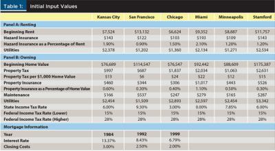
This study used historical financial data from 1984 through 2013 to examine rent-versus-buy decision scenarios for six major metropolitan areas: Kansas City, San Francisco, Chicago, Miami, Minneapolis/Saint Paul, and Stamford/Norwalk (Connecticut). Rent illustrations were based on the applicable rent price index from the Bureau of Labor Statistics for each market.1 Owned-home values were adjusted for each market using the applicable Freddie Mac House Price Index.2 Therefore, the expenses of renting and owning, and house values, mirror the increases and decreases that occurred in each market. Table 1 contains the initial values for each illustration.
This analysis compared rent-versus-buy decisions in the six metropolitan areas for periods of eight, 10, 12, 16, 24, and 30 years—a contrast to previous studies that were limited to eight years (Beracha and Johnson 2012), 10 years (Smith and Smith 2004), and 12 years (Di, Belsky, and Liu 2007).
Following Beracha and Johnson (2012), this study showed net terminal wealth at the end of annual periods. A decision can be evaluated for any desired length of time with the ending wealth at the given year. If ending wealth was positive, renting instead of buying would have been the optimal decision. If ending wealth was negative, buying would have been the optimal decision. If a family chooses to move to another metropolitan area, the ending wealth from selling in their original city can be used as the beginning investment in a subsequent location.
Although net present value is generally employed to evaluate expected future cash flows to arrive at a profitable investment decision, the methodology used in this study analyzed historical cash flows, allowing the calculation of net ending wealth for each scenario for either the rent or buy decision throughout the 30-year period.
Assumptions
In this analysis, it was assumed that the same amount of money was available for either renting or owning. Whichever option was costlier in any given year was taken to be the total amount available for housing for that particular year. Therefore, the difference between the net (after-tax) costs of renting and owning was available for investing in capital markets and accrued toward the total ending wealth for the lower-cost option in each respective year. It is acknowledged as a limitation of this study that this assumption may be unrealistic for many would-be homeowners who are forced to rent due to lack of funds for a down payment on a home; however, using this assumption allowed for a valid comparison of the net ending wealth that either a buy or rent decision would have provided.
Similar to Beracha and Johnson (2012), investment returns accrued from a portfolio were assumed to be composed of 50 percent large company common stocks and 50 percent long-term corporate bonds as reported in Ibbotson’s 2014 Stocks, Bonds, Bills and Inflation. Because investment returns are important to the ending wealth outcome of the rent-versus-buy decision, the effect of an investment portfolio of either 100 percent large stocks or 100 percent corporate bonds was also examined.
For each of the six illustrations presented, it was assumed that the family either rented or owned, and that initial decision was not reversed. This assumption that families do not switch between owning and renting is reasonable. Although some households do switch between owning and renting, the percentage that do so is small (2.3 percent) and the change is often temporary, according to the U.S. Census Bureau’s 2013 American Community Survey, which has the most recent housing and migration data.
Sinai (1997) found the transition from renting to owning was permanent for most people, and for families that did shift from owning to renting, one-third went back to owning within two years. The 2013 American Housing Survey showed only 5.1 percent of all homeowners moved during that year and even fewer became renters. Further, of the 30.8 percent of renters who move annually, only 4 percent become homeowners. Ferreira, Gyourko, and Tracy (2012) dealt at length with housing mobility including temporary-versus-permanent moves between owning and renting. They showed many moves are temporary and that shifts from owning to renting are often reversed within two years. They do not account for seniors specifically moving from owned single-family dwellings into any type of senior housing, whether independent or assisted living.
Calculations and Variables
The calculation of the annual cost of renting is presented by Equation 1.
Rent + Ins + Utilities + Dep = Rent Cost [1]
The variables for Equation 1 are defined as:
Rent = annual rent
Ins = annual property insurance premium
Utilities = annual cost of utilities
Dep = rent deposit paid at beginning of lease (year one only)
Rent Cost = annual cost of renting
These amounts were adjusted from year-to-year according to the applicable index.
The calculation of the annual cost of owning a home is presented by Equation 2.
Trans + Down + Int + Prin + Tax + Ins + Maint + Utilities – TaxSav + Ref – NetRev = Owning Cost [2]
The variables for Equation 2 are defined as:
Trans = transactions costs of home purchase (year one only)
Down = down payment made at purchase (year one only)
Int = annual mortgage interest
Prin = annual mortgage principal paid
Tax = annual property taxes
Ins = annual property insurance premium
Maint = annual cost of home maintenance
Utilities = annual cost of utilities
TaxSav = annual tax savings resulting from deductibility of mortgage interest and property taxes
Ref = refinancing costs (years 1992 and 1999 only)
NetRev = net proceeds from sale
Owning Cost = annual after-tax cost of home ownership
As with the rent equation, these amounts were adjusted from year to year according to the applicable index.
In any given year, the positive difference in the amounts from Equations 1 and 2 was the amount invested each year, contributing to the ending net wealth for the less expensive alternative for that year. If the cost to rent was greater than the cost of owning, the invested difference was allocated to the ending wealth of owning. If the cost of owning was greater in any given year, the invested difference was allocated to the ending wealth of renting. The “net wealth to own” line in the spreadsheet3 includes the net proceeds of the house sale for that year when determining the net wealth to own for a given year. The net advantage to rent does not include the net proceeds from the house sale except in the specific year being analyzed, or, the sale proceeds are counted once in the year of the sale.
Housing characteristics. Recognizing there is a wide variety of housing types in any given market, typical characteristics of owner-occupied and renter-occupied homes were considered to facilitate comparisons and decision-making. The average owner-occupied home in each of the six markets had three bedrooms, and the average rented home had two bedrooms, according to the 2011 and 2013 American Housing Surveys from the U.S. Census Bureau.4 Those surveys also showed that median square footage of owned homes ranged from 1,600 square feet in the New York metropolitan area to 2,000 square feet in Minneapolis and Kansas City, with an average for the six markets of 1,825 square feet. The median rental square footage ranged from 750 square feet in New York to 1,450 square feet in San Francisco. The average for the six metropolitan areas was 1,028 square feet. These averages show that owned homes tended to be larger than rented homes.
Rental information was available for units ranging from zero to four bedrooms. To compensate for the differences in the average number of bedrooms and square footage between rented and owned homes, and to narrow the lifestyle gap between renting and owning, costs applicable to a four-bedroom rented apartment were compared to the costs of a three-bedroom owned home. By doing so, the costs of each were more representative of equivalent living space.
Rent. Annual rent was the median annual rent for a four-bedroom apartment as reported by the Department of Housing and Urban Development, 2015 data.5 Rent was adjusted annually for each market according to the applicable Metropolitan Rent Price Index from the Bureau of Labor Statistics’ Consumer Price Index for All Urban Consumers, Rent of Primary Residence. A rental deposit equal to two months’ rent was included in the analysis at the commencement of the lease.
Owned home value. Acknowledging there are varying estimates for home values in any given market, this study used median, three-bedroom home prices reported by the National Association of Realtors in its Metropolitan Median Area Prices and Affordability report, and adjusted annually by the Freddie Mac House Price Index.6
Mortgage expense. This study employed typical mortgage terms that existed from 1984 to 2014. Principal and interest payments were based on an 80 percent loan-to-value, 30-year, fixed-rate conventional mortgage as reported by Freddie Mac in the Primary Mortgage Market Survey7 for January of the applicable year.
This analysis assumed that homeowners refinanced when rates fell. The average mortgage interest rate in January 1984 was 13.37 percent. Therefore, refinancing was assumed to occur in January 1992, at 8.43 percent, and again in January 1999, at 6.79 percent. Although the refinancing decisions in the scenarios are somewhat arbitrary and capture some of the lowest rates available, they were consistently applied in all six scenarios.
The amounts for points were included for the original loan in 1984, and for refinancing in 1992 and 1999, and were based on the average number of points reported by Freddie Mac.8 These were 2.3, 1.8, and 0.9, respectively. Homeowners deducted interest payments at assumed federal income tax rates (15 percent for the first set of scenarios; 28 percent for the second set of scenarios). Homeowners also deducted interest payments at the applicable state income tax rate.
Utilities. Utility expenses were estimated for each of the six metropolitan areas using the U.S. Census Bureau’s American Housing Survey tables, and were adjusted annually using the Bureau of Labor Statistics’ Household Energy Price Index.9
Property insurance. Property insurance costs were estimated as a percentage of rent paid for renters or of home value for owners. The applicable percentages were estimated from the latest available data [at the time of this writing] from the U.S. Census Bureau’s American Housing Survey tables for each market. The premium for renters was based on an HO-4 policy, and for owners it was based on an HO-3 policy. For example, the annual cost of property insurance in Kansas City was approximately 2 percent of annual rent, and for homeowners it was approximately 0.6 percent of home value.
Property taxes. Renters have no separate property tax expense; property taxes are implicitly included in the rent charged by the landlord. Property taxes for homeowners were estimated for each market based on the average property tax rate applicable for that area. Property tax rates were taken from the U.S. Census Bureau’s American Housing Metropolitan Survey.
The tax rate was assumed to be stable over the study period, based on the latest available rate. Home values were multiplied by this rate to determine the annual property tax expenditure. A planner may input the applicable property tax rate, as a millage rate per $1,000 of valuation, for any locality in cell F40 in the spreadsheet (located at realestate.uni.edu/research-papers-articles-informative-writing#). The formulas in the spreadsheet will automatically incorporate the applicable rate in the final calculations. Property tax deductions were calculated using assumed federal income tax rates of both 15 percent and 28 percent, and at the applicable state income tax rate.
Maintenance and repair costs. Costs of maintenance and repairs were not included as a separate expense for renters, because they are commonly the responsibility of the landlord who implicitly includes these costs in the rent charged. For homeowners, annual maintenance and repair costs were estimated using average maintenance costs provided by the Bureau of Labor Statistics Consumer Expenditure Survey for the years 2003 through 2013.10 The average annual rate of change for this 10-year period was applied to each year of the 30-year study period to estimate annual costs.
Results and Analysis
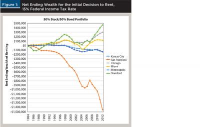
Table 2 presents net ending wealth figures at various periods up to 30 years and at assumed federal tax rates of 15 percent and 28 percent. The results using a 15 percent tax rate and decision horizons of eight years, 10 years, and 12 years show renting was the better decision in five of the six markets, the one exception being San Francisco. However, the results for longer-term periods of ending wealth methodology differ markedly from the shorter terms with longer periods tending to favor home ownership. Nevertheless, 30-year net ending wealth still favored renting for three of the six scenarios: the metropolitan areas of Stamford, Chicago, and Miami.
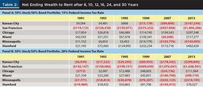
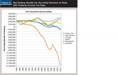
As Table 2 shows, the benefits of owning versus renting increase with tax brackets. When the same six scenarios were revisited using a 28 percent tax rate, the net ending wealth for choosing to rent was decidedly lower in every scenario. Because some of the costs of home ownership are deductible, most notably mortgage interest and property taxes, tax savings were greater for homeowners in higher federal and state tax brackets. For one metropolitan area, Miami, home ownership became more favorable than renting when the tax bracket increased from 15 percent to 28 percent.
Figure 1 and Figure 2 show the evolution of the two different tax bracket scenarios in graphical form.
The scenarios presented in Table 2 incorporate an investment portfolio composed of 50 percent corporate bonds and 50 percent equities. Because the returns to the lower-cost alternative going forward were important to the scenario outcomes, this analysis reexamined the scenarios where investment portfolios consisted of either 100 percent bonds or 100 percent stocks.
Over each of the periods presented in Table 2, the stock portfolio outperformed the bond portfolio. For the entire 30-year period, the annualized geometric mean return for the stock portfolio was 11.1 percent, notably higher than the 9.4 percent produced by the bond portfolio. Because the rent decision tended to produce greater early cash flows available for investing, the higher returns afforded by the all-stock portfolio favored the decision to rent for every metropolitan area except San Francisco. However, assuming a 100 percent stock investment portfolio over a portfolio evenly split between stocks and bonds did not change the outcome of any of the dozen 30-year scenarios presented in Table 2.
Comparing Two Extreme Scenarios
To better understand the factors that have driven these results, it is instructive to contrast the best renting scenario, Stamford, Connecticut, with net ending wealth of $462,629, and the best buying scenario, San Francisco, with net ending wealth of $1,456,296 (assuming a federal tax rate of 15 percent, a 50 percent equity/50 percent debt investment portfolio, and a 30-year holding period).
The main factors seemed to be initial rental costs and housing values, and the trajectory of housing and rent prices during the holding period. Smith and Smith (2004) accounted for the relative change in rents and mortgage payments, but not for how the beginning levels might affect the results. In 1984, the median price of a three-bedroom home in Stamford was $175,387, while the median price in San Francisco was a relatively inexpensive $114,547. Over the next 30 years, however, median three-bedroom home values in San Francisco increased by 393 percent to slightly more than $450,000. The median three-bedroom home value in Stamford increased to $520,000, but because of the higher initial starting point the rate of increase was lower at 296 percent. The very large gain in housing prices in San Francisco made a substantial contribution to ending wealth.
The relative changes in rents also affected the results. Rents were increasing in both San Francisco and Stamford, and similar to what was happening to house prices, rent increased at a higher rate in San Francisco than it did in Stamford. Over the 30-year period, rent in San Francisco increased threefold, at an average annual rate of nearly 12 percent, compared to an average annual rate of 8.8 percent in Stamford.
The combination of larger relative increases in house prices and rent in San Francisco resulted in a much larger accumulation of ending wealth from owning in San Francisco. Although mortgage interest rates were high in 1984, the San Francisco homeowner could lock in monthly mortgage payments of approximately $1,064. Even though property taxes were ever increasing, these monthly payments remained relatively stable, and were even reduced by subsequent refinancing. While home values and rent had both increased in Stamford, the increase in home values was not sufficient to offset the increase in rent.
Together, these two factors made home-buying in San Francisco financially much more preferable to renting, and made renting in Stamford preferable to buying. The impact of these factors is seen in ending wealth because of the better decision of freeing funds for debt and equity investment.
In San Francisco, the advantage toward renting, largely because of the initial down payment on the home, only lasted one year. The difference was invested in equities and bonds for the next 29 years. In Stamford, however, the advantage to renters lasted a decade, with the renting advantage difference accruing toward capital markets investments.
Conclusion
For many families, a home represents their largest single asset. Consequently, the decision to rent or buy takes on significant importance. This decision has been studied from several perspectives. Although important non-financial factors may dictate a family’s final decision, this study focused on net ending wealth resulting from the initial decision to either rent or buy a home.
This study enables evaluation of the rent-versus-buy decision for holding periods from one year to 30 years. The basis for the decision is long-term ending wealth as a single number that is easily understood. Contrary to previous studies that have consistently supported home ownership as the more desirable decision, this study’s results from an ending wealth perspective using historical data demonstrated that the optimal decision was not always home ownership.
Further, an ending wealth decision rule indicates the better decision will often change from one year to the next as the scenarios evolve. The optimal decision from an ending wealth perspective is highly dependent upon on the time horizon, with a shorter time horizon generally favoring the decision to rent.
Because of the favorable tax treatment of home ownership, higher federal and state tax brackets always favor buying over renting. High investment returns, which are generally (but not always) unpredictable, also favor the decision to rent rather than buy.
Nevertheless, individual market conditions cause the optimal decision in some markets to favor renting and in other markets to favor owning, even over a 30-year time horizon. In some markets the difference in ending wealth between renting and owning was substantial, amounting to nearly $1.5 million in the San Francisco market.
Implications for Financial Planners
Financial planners should be attuned to their clients’ needs and desires regarding non-financial considerations; however, they should also be able to offer advice regarding the financial implications of the rent-versus-buy decision.
An important result of this study is that, contrary to common belief, ending wealth has not always been maximized by purchasing a home. The financial outcome for the rent-versus-buy decision is influenced by a number of factors, the most important of which are: (1) the time frame being considered; (2) the client’s tax bracket; (3) the relative price changes between the housing and rental markets for the particular area; and (4) the prospect for returns in capital markets.
Although ending wealth could be monitored for shorter time periods within the 30-year sample, many, if not most, potential homeowners will not adopt an all-in approach to this decision. It is also quite likely that non-financial factors will be even more important to a client’s decision.
Suppose a client has decided to buy a home based mainly on non-financial factors, but is unsure whether to proceed now or later. For a situation such as this, the financial factors identified by this study should be helpful.
Because shorter holding periods tend to favor renting over buying, clients who are unsure about the amount of time they will be able to live in a certain location might be advised to wait until this uncertainty is resolved.
Since a higher tax bracket weighs in favor of the decision to purchase, clients in the higher tax brackets might be advised to purchase a home to capitalize on the benefits of property tax and mortgage interest deductions. Rapidly accelerating markets for home rental and sales could also be a factor in favor of an earlier rather than later decision to purchase.
While high investment returns seem to generally favor the decision to rent, future capital market returns are notoriously difficult to predict, especially in the short term.
Because each of these factors is difficult to predict, it is impossible for financial planners to say for certain whether the superior ending wealth outcome will result from renting or from buying; however, understanding the factors that contribute to the final financial outcome is essential to providing competent advice.
Endnotes
- Bureau of Labor Statistics’ Consumer Price Index for All Urban Consumers, Rent of Primary Residence, 1984–2014, available at data.bls.gov.
- The Freddie Mac House Price Index is available at freddiemac.com/research/docs/msas_new.xls.
- Access the spreadsheet at realestate.uni.edu/research-papers-articles-informative-writing#.
- The 2011 metropolitan survey tables are available at census.gov/programs-surveys/ahs/data/2011/ahs-2011-summary-tables/ahs-metropolitan-summary-tables.html. The 2013 survey tables are available at census.gov/programs-surveys/ahs/data/2013/ahs-2013-summary-tables.html.
- Department of Housing and Urban Development 50th Percentile Rent Estimates are available at HUDuser.org/portal/datasets/50per.html.
- The National Association of Realtors 2017 Metropolitan Median Area Prices and Affordability report is available at realtor.org/topics/metropolitan-median-area-prices-and-affordability. The Freddie Mac House Price Index is available at freddiemac.com/research/docs/msas_new.xls.
- Freddie Mac mortgage interest rate and fee data is available from freddiemac.com/pmms.
- See “30-Year Fixed-Rate Mortgages Since 1971” at freddiemac.com/pmms/pmms30.html.
- See the Bureau of Labor Statistics’ Consumer Price Index for All Urban Consumers, Household Energy, 1984–2014, at data.bls.gov.
- The Bureau of Labor Statistics’ Consumer Expenditures data is available at bls.gov/opub/reports/consumer-expenditures/2014/home.htm.
References
Beracha, Eli, and Mark Hirschey. 2009. “When Will Housing Recover?” Financial Analysts Journal, 65 (2): 36–47.
Beracha, Eli, and Ken Johnson. 2012. “Lessons from Over 30 Years of Buy versus Rent Decisions: Is the American Dream Always Wise?” Real Estate Economics 40 (2): 217–247.
Case, Karl, and Robert Shiller. 2004. “Is There a Bubble in the Housing Market?” Brookings Papers on Economic Activity 2: 299–342.
Di, Zhu Xiao, Eric Belsky, and Xiaodong Liu, 2007. “Do Homeowners Achieve More Household Wealth in the Long Run?” Journal of Housing Economics 16 (3-4): 274–290.
Ferreira, Fernando, Joseph Gyourko, and Joseph Tracy. 2012. “Housing Busts and Household Mobility: An Update.” Federal Reserve Bank of New York Economic Policy Review 18 (3) 1–15.
Martin, Robert. 2008. “Housing Market Risks in the United Kingdom.” International Finance Discussion Papers, Number 954. Board of Governors of the United State Federal Reserve System: Washington, D.C.
McCarthy, Jonathan, and Richard W. Peach. 2004. “Are Home Prices the Next Bubble?” Federal Reserve Bank of New York Economic Policy Review 10 (3): 1–17.
Sinai, Todd. 1997. “Taxation User Cost and Household Mobility Decisions.” No. 303. Wharton School Samuel Zell and Robert Lurie Real Estate Center, University of Pennsylvania.
Smith, Margaret, and Gary Smith. 2004. “Is a House a Good Investment?” Journal of Financial Planning 17 (4): 68–75.
Stults, Rachel. 2015. “Where Is Buying Much Better Than Renting? In the 10 Cities Our Data Team ID’d.” Available at realtor.com/news/trends/buying-better-than-renting-10-cities.
Citation
Cox, Arthur, and Richard Followill. 2018. “To Rent or Buy? A 30-Year Perspective.” Journal of Financial Planning 31 (5): 48–55.