An Intuitive Examination of Downside Risk

Journal of Financial Planning: June 2013

Executive Summary

• This paper offers insight regarding several unresolved issues related to downside risk evaluation. Specifically, we provide clarity to semivariance, which is a well-known, but often misunderstood risk measure.
• We examine the calculation methodology for both semivariance and semideviation and give practical financial planning interpretations.
• Semideviation is used in the Sortino ratio, which assesses return per unit of downside risk. The Sortino ratio is pervasive and well understood, but we question whether a majority of practitioners can make an accurate calculation of the semideviation measure.
• Popular asset class returns from 1926–2011 are examined, and we find that while small company stocks and large company stocks have similar Sharpe ratios, small stocks have superior Sortino ratios.
• The information ratio is an important measure of active fund manager performance. We suggest replacing the standard deviation of active return with the semideviation. A real-world example demonstrates the value of this revised metric.

Kenneth M. Washer, D.B.A., CFP^®, CFA, CPA (inactive) is an associate professor of finance at Creighton University in Omaha, Nebraska. He has published more than 30 papers in various journals. (KenWasher@creighton.edu)
Robert R. Johnson, Ph.D., CFA, CAIA, is a professor of finance at Creighton University in Omaha, Nebraska. He has published more than 65 papers in academic and practitioner journals.
(RRJohnson@creighton.edu)
The recent financial crisis, coupled with the increasing prominence of alternative assets whose returns typically have asymmetrical distributions, has led to a greater focus on the concept of risk measurement, and in particular, downside risk measurement. While downside risk measures are increasingly relied upon by investment professionals, several issues remain unresolved regarding how to properly implement the measures.
Financial professionals have likely been exposed to semideviation (the square root of semivariance) in principle, but may be confused by the variations of the measure that are presented. Certainly, the interpretation is not as simple as that of standard deviation or variance measures. The interpretation is not only important in practice, but the finance literature often employs the measure in empirical studies (for example, see Beach (2006), Chevallier and Sévi (2012), Gordon (2003), Kurgin (2002), and Regan (1993)).
The popular textbook written by Maginn, Tuttle, McLeavey, and Pinto (2007), Managing Investment Portfolios, makes four mentions of downside risk, downside deviation, and semivariance. Maginn et al. acknowledge the use of downside risk measures in practice, but do not discuss the calculation in any detail. This shortcoming is common in other textbooks as well. The student/practitioner is given little help in the application of these measures. Likewise, Investment Analysis and Portfolio Management (Reilly and Brown 2011) devotes one paragraph to semivariance but does not provide a formula. We believe downside deviation is a useful risk measure that can help advisers make better investment decisions, and as such, a more explicit description of the concept is warranted.
In this paper, we take an intuitive approach to calculating and interpreting semivariance and semideviation. We also examine two ways these measures can be used in practice. We review the Sortino ratio, which is a measure of excess return per unit of semideviation. Lastly, we contend that the information ratio can be improved by dividing mean active return by the semideviation of active return, instead of the standard deviation of active return.

Variance and Semivariance

To understand semivariance, one must first understand variance, the preeminent measure of total risk in finance. Equation (1) shows the variance formula as applied to a sample of historical returns.

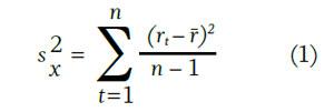
In the above formula, rt is the return in period t, is the average return over the entire period, and n is the total number of periods in the sample. In other words, the variance is equal to the sum of the squared deviations divided by the number of observations minus one. The positive square root of the variance is the standard deviation, which is helpful in determining the probability of certain outcomes. For example, if one assumes a normal distribution, probabilistic statements can be made such as “68.3 percent of all outcomes fall within plus or minus one standard deviation of the mean.” Likewise, if no assumption is made about the underlying return distribution, Chebyshev’s inequality states that at least 75 percent of all outcomes are within two standard deviations of
the mean.¹

If only negative deviations are squared and summed in the numerator, equation (1) also may be applied to the semivariance calculation. In essence, all positive deviations are set to zero and do not affect the summation. Thus, if the return in period t is less than the average return, the difference is squared and the numerator increases. However, if the return is above average, the difference is set to zero and the numerator does not increase. An analyst may decide to use a target return instead of the mean return (r) in the calculation.

The intuition behind semivariance is straightforward: above-average returns do not increase risk, as outperformance is beneficial to the investor.

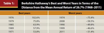
Warren Buffett’s Berkshire Hathaway provides a good example. From 1968 to 2011, the average annual return on the stock was 26.7 percent.² Berkshire’s best five years and worst five years are shown in Table 1 as deviations from the mean. One can see that in terms of absolute value, the five largest positive deviations are more extreme than the five largest negative deviations. However, these positive “outliers” significantly raise the variance of Berkshire’s return. In this case, the variance is 0.1330 and the semivariance is 0.0519. The ratio of semivariance to variance is 0.39, which indicates that downside risk effectively comprises only 39 percent of total risk. One logically concludes that the variance and standard deviation measures in Berkshire’s case actually overestimate risk. We believe that for asymmetrical distributions, the financial professional ignores significant information when using variance or standard deviation as the sole measure of risk.

The most contentious aspect to the semivariance formula is the denominator n–1. The CFA Institute text, Quantitative Investment Analysis (DeFusco et al. 2007), instructs candidates to divide the sum of the squared deviations by n–1, where n is defined as the number of downside deviations.³ It appears logical that if there are 20 negative deviations, one should divide by 19 to get the average length of a downside, squared deviation. However, this is not the case. One should divide by the total number of observations (negative and positive deviations) minus one. This is the procedure that Nobel Laureate Harry Markowitz posited in Chapter 9 of his seminal work, Portfolio Selection: Efficient Diversification of Investments.⁴

Confusion perhaps can be alleviated by focusing on the name “semivariance” and remembering that “semi” means “partly.” So, dividing by one less than the number of all observations gives a downside squared deviation that is a portion of the variance. In our analysis presented below, semivariance ranges from 34 percent (intermediate-term government bonds) to 55 percent (large company stocks) of the variance.

Interpreting and Using Semivariance

We use historical returns on various asset classes and descriptive statistics to show the usefulness of the semivariance statistic. Annual return data from 1926 through 2011 were collected from Ibbotson’s Stocks, Bonds, Bills and Inflation: 2011 Yearbook. The asset classes include large company stocks, small company stocks, long-term (LT) corporate bonds, long-term government bonds, intermediate-term (IT) government bonds, and Treasury bills. Table 2 displays descriptive statistics for the asset classes.

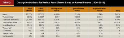
As shown in Table 2, small stocks have the highest average return (16.51 percent) and also the highest standard deviation (32.51 percent). It should be noted that we did not test for statistical significance, as our main goal was making meaningful interpretations of the results. The only asset class that appears to be dominated in mean-variance space is long-term government bonds as this asset class has a lower average return and higher standard deviation than long-term corporate bonds. Notice, this asset also is dominated on the basis of ­semideviation, as the semideviation of long-term government bonds is higher than that of long-term corporate bonds.⁵

Financial professionals should be aware of several benefits to using semivariance. First, the ratio of semivariance to variance indicates the portion of the variance emanating from the left side of the distribution.⁶ For example, this ratio is 55 percent for large company stocks, indicating that 55 percent of the variance is on the left side of the distribution. Thus, downside deviation is responsible for 55 percent of total deviation. When the distribution is skewed to the left (skewness is −0.37 for large company stocks), semivariance is almost always greater than 50 percent of the total variance, and, we contend, variance underestimates risk.
It also should be noted that all asset classes other than large stocks have ratios of semivariance to total variance that are less than 50 percent. This indicates that during this period, variance and standard deviation effectively overstated downside risk for these asset classes.

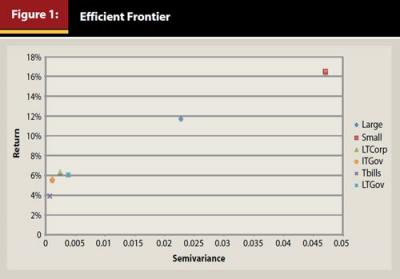
Semivariance also can be used to compare securities based on a mean/semivariance framework, preferring assets or portfolios with higher means and lower semivariances, all else being equal. The ratio of return per unit of semivariance can be calculated for various securities, and an efficient frontier can be plotted as shown in Figure 1. Figure 1 reveals that long-term government bonds (LTGov) are dominated by long-term corporate bonds (LTCorp). This mean/semivariance framework does not extend to portfolio construction as covariances between securities are of utmost importance.

An advantage associated with the use of standard deviation is that probabilistic statements can be made. This cannot be done with semideviation. For example, if the analyst assumes small stocks are normally distributed, he or she can make a probability statement such as “68.3 percent of actual annual returns will fall within the range of −16.00 percent to 49.02 percent” (average return for small stocks of 16.51 percent ± 1 standard deviation of 32.51 percent). One cannot use semideviation to make a similar probability statement.

The Sortino Ratio

The Sortino ratio is closely affiliated with the Sharpe ratio. The Sortino ratio places excess return (return above the risk free rate or some target rate) over the semideviation. A higher value indicates a more desirable security or portfolio, holding all else constant. Equation (2) shows the formula for the Sortino ratio (SR):

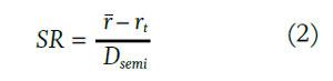
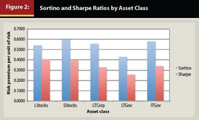
In the formula, r is the average return, r₁ is the target return, and D_semi is the semideviation. The Sharpe ratio is identical to equation (2) except that the standard deviation replaces the semideviation in the denominator. Equation (2) is a discrete time formula for the Sortino ratio. For the continuous time formula, see Sortino and Satchell (2001). Figure 2 displays the Sortino and Sharpe ratios for large stocks, small stocks, long-term corporate bonds, long-term government bonds, and intermediate-term government bonds. Large company stocks and small company stocks have equivalent Sharpe ratios, but the Sortino ratio is higher for small stocks. This implies that investors have historically received higher excess returns per unit of downside risk from small stocks versus the other asset classes, a key benefit of small stocks.

Long-term corporate bonds and intermediate-term government bonds have Sortino ratios that are between large and small stocks. However, the Sharpe ratios of these two fixed-income sectors are much lower than Sharpe ratios of the two equity classes.
 

In discussing the Sortino and Sharpe ratios, Maginn et al. (2007, 633) wrote:
A side-by-side comparison of rankings of portfolios according to the Sharpe and Sortino ratios can provide a sense of whether outperformance may be affecting assessments of risk-adjusted performance. Taken together, the two ratios can tell a more detailed story of risk-adjusted return than either will in isolation, but the Sharpe ratio is better grounded in financial theory and analytically more tractable. Furthermore, departures from normality of returns can raise issues for the Sortino ratio as much as for the Sharpe ratio.

The Sharpe ratio for both large and small company stocks is 0.40. If we also factor in the Sortino ratio, we see that large stocks have a lower Sortino ratio than small stocks (0.54 versus 0.59). In combination, these ratios indicate that, somewhat counterintuitively, the downside risk is less for small stocks, or alternatively, large positive deviations from the mean contribute more to the variance of small stocks than large stocks.

In the following section, we discuss the information ratio and how replacing the standard deviation with semideviation in this common measure can provide additional information to the adviser choosing an actively managed fund.

Modified Information Ratio

The information ratio (IR) often is used to analyze active return. Equation (3) shows the formula for IR.

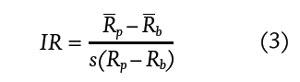
 The numerator represents active return and is the difference between the mean return of the portfolio (R_p) and the mean return of the benchmark portfolio (R_b). The denominator is the standard deviation of active return (s(R_p – R_b)).
This measure is often useful when evaluating the performance of an active manager as it indicates the consistency of active return. A higher IR is preferred to a lower one. This measure is most appropriate when active return is a normally distributed variable. If a fund’s active return distribution is skewed to the right, the manager may contend that the standard deviation of the active return is too high and that the information ratio is too low.

To account for this potential problem, IR can be modified by employing the semideviation of active returns in the denominator. We call this the modified IR (IR_mod). This measure gives an indication of active return per unit of downside risk. The relationship between IR and IRmod is very similar to the relationship between the Sharpe ratio and the Sortino ratio.

Table 3 shows the active return and information ratios for two highly rated mid-cap value funds, specifically the Artisan Mid Cap Value Investor Fund (ARTQX) and the Nicholas Equity Income I Fund (NSEIX) . The underlying 20 quarterly returns (2007–2011) were gathered from Morningstar.com. Both funds earned five-star ratings from Morningstar. The benchmark return used was the mid value category average return.
 

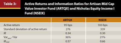
Both funds outperformed the benchmark by approximately 100 basis points per quarter over this period. Based on the traditional information ratio, ARTQX is preferred, as it earned 0.34 basis points of excess return per unit of risk versus 0.30 for NSEIX. However, the ratio of semivariance to variance indicates that the variance measure overestimates risk for each fund, and because of this, the semideviation is a better risk measure. In fact, we find that our preference for funds changes when semideviation is substituted for standard deviation in the IR formula. NSEIX is the superior fund, as the modified IR is higher (0.66) than ARTQX’s modified IR (0.57). This example clearly indicates the importance of including semivariance/semideviation in the analysis of securities. It is not an overriding measure, but one that should be considered complementary to traditional risk measures.

Conclusions

In this paper we have shown how financial professionals can calculate and implement the semivariance measure into their analytical work. The literature provides very little guidance in this area. The ratio of semivariance to variance gives an idea of the symmetry of the distribution.

 The square root of semivariance is semideviation, which is most notably used in the Sortino ratio. This ratio is excess return (return above average or some target level) divided by the semideviation. The Sortino and the Sharpe ratios are more likely to rank securities differently when the ratio of semivariance to variance diverges substantially from 50 percent. One could argue the Sortino ratio is superior to the Sharpe ratio, but many advisers use the two measures in con­junction. This paper also introduced the information ratio, which is a measure often used in assessing a fund manager’s performance. It is equal to average active return divided by the standard deviation of active return. We suggest that this measure can be improved by substituting semideviation for standard deviation. A practical example demonstrates that the two information ratios can rank funds differently when the distribution of active return is skewed.
A primary objective of many financial professionals is to properly manage the risk/return tradeoff. Understanding measures of downside risk such as semivariance, semideviation, Sortino ratio, and modified information ratio is critical to making optimum investment decisions.

Endnotes

1. Chebyshev’s inequality says that no matter the shape of the distribution, the minimum percentage of observations that fall within k standard deviations of the mean is 1 – 1/k2. Thus, at least 75 percent of the observations will fall within two standard deviations of the mean (1 – 1/22).
2. Market returns for Berkshire Hathaway back to the 1960s were unattainable from traditional databases. We used http://allfinancialmatters.com/2008/04/02/a-look-at-berkshire-hathaways-annual-market-returns-from-1968-2007/ and employed Yahoo’s finance site to calculate returns for 2008–2011. The compound average growth rate (CAGR) over the entire period was 21.7 percent, which is in line with the 20.3 percent CAGR Warren Buffett reported in the 2009 shareholder’s letter.
3. The 2012 CAIA curriculum instructs candidates to divide by T, the number of negative deviations.
4. Markowitz used n as the denominator (not n–1) in Chapter 9 of Portfolio Selection: Efficient Diversification of Investments, which is correct if one is calculating semivariance based on a population. Our illustrations assume a sample. For large samples there is no significant difference between the two approaches.
5. Treasury bonds are dominated by other asset classes on a before-tax basis; however, because their interest is exempt from state and local income taxes, they may not be on an after-tax basis.
6. The denominators used in the semivariance and variance calculations are either both n (population) or n–1 (sample). When you take the ratio of semivariance to variance, the n (or n–1) denominators cancel each other out.
   
   

References

Beach, Steven L. 2006. “Why Emerging Market Equities Belong in a Diversified Investment Portfolio.” The Journal of Investing 15 (4): 12–18.
Chevallier, Julien, and Benoît Sévi. 2012. “On the Volatility-Volume Relationship in Energy Futures Markets Using Intraday Data.” Energy Economics 34 (6): 1896–1909.
DeFusco, Richard A., Dennis W. McLeavey, Jerald E. Pinto, and David E. Runkle. 2007. Quantitative Investment Analysis, 2nd ed. Hoboken, New Jersey: John Wiley & Sons.
Gordon, David. 2003. “Risk by Any Other Name.” The Journal of Alternative Investments 6 (2): 83–86. Ibbotson Associates. 2011. Stocks, Bonds, Bills, and Inflation: 2011 Yearbook. Chicago, Illinois: Morningstar.
Kurgin, Vladislav. 2002. “Value Investing in Emerging Markets: Risks and Benefits.” Emerging Markets Review 3 (3): 233–244.
Maginn, John L., Donald L. Tuttle, Dennis W. McLeavey, and Jerald E. Pinto. 2007. Managing Investment Portfolios: A Dynamic Process, 3rd ed. Hoboken, New Jersey: John Wiley & Sons.
Markowitz, Harry. 1959. Portfolio Selection: Efficient Diversification of Investments. New Haven, Connecticut: Yale University Press.
Regan, Patrick J. 1993. “Pension Fund Perspective: Analyst, Analyze Thyself.” Financial Analysts Journal 49 (July/August): 10–12.
Reilly, Frank, and Keith Brown. 2011. Investment Analysis and Portfolio Management, 10th ed. Independence, Kentucky: Cengage Learning.
Sortino, Frank, and Stephen Satchell. 2001. Managing Downside Risk in Financial Markets: Theory, Practice, and Implementation. Oxford, UK: Butterworth-Heinemann, Quantitative Finance Series.

Citation

Washer, Kenneth M., and Robert R. Johnson. 2013. “An Intuitive Examination of Downside Risk.” The Journal of Financial Planning 26 (6): 56–60.