Journal of Financial Planning: July 2014
Haiwei Chen, Ph.D., CFA, is a visiting assistant professor of finance at John Carroll University. He received a Ph.D. in economics from Emory University.
Jim Estes, Ph.D., CFP®, ChFC®, CLU®, CPCU, is a professor of finance at California State University, San Bernardino, a principal of Alpha Wealth Management, and a FINRA arbitrator. He has worked with the California and Texas legislatures on bills relating to municipal bonds.
Daniel Jubinski, Ph.D. is a tenured assistant professor of finance at Saint Joseph’s University. He received a Ph.D. from the University of Virginia.
Executive Summary
- This paper explores the ramifications of mutual fund and money manager municipal bond benchmark choices.
- The ramifications of the selection of an index by a mutual fund or money manager that results in a favorable comparison is explored in light of FINRA guidelines.
- Two primary measures could be used as benchmarks: the Merrill Lynch Index and the Barclays Capital Index. Almost all funds examined in this study pick the Barclays Capital Index as the benchmark.
- While 60 percent of funds beat the Barclays Capital Index, less than 48 percent beat the Merrill Lynch Index.
- Although most financial planners do not select their own index as a benchmark, they should be aware of other indexes that may more accurately reflect the performance of their selected investment instruments and disclose that difference to a client in regular investment reviews.
Acknowledgements: The authors thank Thanh Ngo, Shan Yan, and two anonymous referees for helpful comments.
The municipal bond fund industry differs from many other sectors in two aspects. First, the majority of the fund investors are high net worth (HNW) individuals. These investors are viewed as more sophisticated with the education to understand the risks of their investments and the means to hire professional financial advisers. Secondly, unlike many other sectors, the municipal bond market has two well-established market indexes: the Barclays Capital Municipal Bond Index (BC Index) and the Bank of America Merrill Lynch Municipal Securities Master Index (ML Index).
Despite the importance of these two benchmarks, there are fewer fund-level studies that examine the application of these benchmarks and the implications of using the one that would appear to enhance performance. Few studies exist that examine the choice of alternative benchmarks on the performance evaluation of fund managers in the municipal bond fund industry. Jakob and Costa (2011) found that a totally different set of calculations needs to be used in equity fund comparisons to more accurately assess manager performance relative to their benchmark, no matter what index was selected by the manager.
This paper explores a marked difference in the two alternative benchmarks and questions whether or not the appropriate benchmark matching fund holdings is being used.
This study documents that the monthly returns of the BC Index are consistently lower than the returns of the ML Index and that individual fund returns are equally correlated with both index returns. These findings indicate that the ML Index could be used as a benchmark. Yet, long-term national municipal bond funds overwhelmingly pick the BC Index as the benchmark. Such a deliberate choice of the benchmark distorts the performance evaluation picture in favor of fund managers at the expense of fund investors. Currently, 60 percent of the funds beat the BC Index each year, whereas less than 48 percent of the funds beat the ML Index. Advisers bear a significant responsibility to be aware of differences and accuracy of benchmarks and explain these differences to their clients.
This paper describes the differences in the two indexes, then reviews related studies and explains the research design of the study. Data and hypotheses are then presented with empirical results.
Municipal Bond Market Indexes
Panel A of Table 1 provides a comparison of the two indexes, which have several similarities. For example, both include investment-grade bonds based on the average of the three U.S. bond rating agencies. Both indexes include bonds with a maturity of at least one year. Both indexes are total-return indexes. The BC Index started in 1980. The ML Index started in 1988. The main difference between the two is the market value at issuance. The BC Index includes more small-sized bond issues than the ML Index. The BC Index requires a minimum market value of $7 million for an issue to be included; in contrast, the ML Index only includes those bonds with a minimum market value of $10 million at the time of inclusion1.
Many issues are less than $10 million. For example, Robbins and Simonsen (2013) reported that 40 percent of all issues by municipalities in California (the largest among all states issuing municipal bonds) were below $10 million between 2007 and 2009. As a result, there are more bonds in the BC Index. One can argue that the BC Index is more representative than the ML Index. However, small bond issues tend to have lower liquidity than larger issues. This is important for mutual funds and individuals who are large holders of municipal bonds. The smaller or more thinly traded municipal bonds tend to be issued by smaller municipalities and purchased by individual investors who are familiar with the municipality or the bond issue.
The distinct lack of liquidity, establishing a ready price for resale coupled with the small issue, is usually not workable for larger mutual funds that may require a larger position in rebalancing or replacing called or sold issues. Thus, while the BC Index includes smaller issues and does indeed give it a wider representation, this does not truly represent the profile of most municipal bond funds. A check of the top 100 largest municipal bond funds (those with total net asset value greater than $273 million at the end of September 2013) in the United States shows an average size holding of $2.45 million. It is $1.67 million for the top 200 funds (those with total net asset value greater than $97 million at the end of September 2013). Logic shows that to take a position on an issue under $10 million would entail a larger concentration of risk in a small issue than would be prudent.
Municipal bonds are typically held to maturity by investors with few trades one month after the issue. For example, Ang and Green (2011) reported that “the average municipal bond trades only twice per year, with 5 percent of securities trading only once over 12 years” (p. 10). Bonds from a small size issue will more likely be subject to a stale price bias resulting from fewer trades. If small issuances would most likely be bought by a few individuals or firms, or be scattered (insignificantly in overall value) among many funds, the ML Index may be more representative of all funds.
How closely are the returns of the two indexes related? Panel B of Table 1 shows that the ML Index has a higher average monthly return than the BC Index in eight of the months represented, although the differences are statistically insignificant. The BC Index has a higher average return in January and April, although the relationship is not statistically significant. Figure 1 shows that there is no significant change in such a pattern over time.
Note that the average return in January is much higher for the ML Index than for the BC Index. Under the January effect hypothesis, more sophisticated investors, on advice from tax or investment professionals, sell holdings of losing securities in December to harvest capital losses. These investors then reinvest the sale proceeds in January, which results in a positive return in January. Thus, the two indexes tell two tales of return seasonality for the municipal bond market.
Panel C of Table 1 presents findings when monthly returns are regressed on a January dummy variable. This test was made to determine whether returns are higher in January than in other months. The dummy variable is insignificant in the ML regression but significantly positive in the BC regression. This result may be a reflection of the inclusion of smaller issue of bonds in the BC Index.
Performance Evaluation: The Role of Benchmarks
Although the Securities and Exchange Commission requires that mutual funds present a benchmark to enable investors to judge the relative performance of a fund, the actual choice of the benchmark is left up to individual fund managers. It is certainly possible that a fund manager could strategically choose a more favorable benchmark to artificially enhance his or her performance.
Lehmann and Modest (1987) found that the performance ranking within a sample of 130 mutual funds changes dramatically when different benchmarks are used. Similarly, Grinblatt and Titman (1994) showed that alternative benchmark choices can produce very different results in fund performance evaluation. Ackermann, McEnally, and Ravenscraft (1999) showed that hedge funds underperform market benchmarks. Sensoy (2009) showed that managers of equity funds purposely select a favorable benchmark.
Intuitively, if investors who use professional advisers are more sophisticated than average investors, one would expect less opportunistic behavior on the part of managers, because such behavior would not be tolerated by their sophisticated clientele. One would also expect that professional advisers are aware of appropriate benchmarks and would discuss these issues with their clients. The hypothesis that a practice of selecting an easy benchmark in the municipal bond fund industry is less prevalent is tested. In this regard, the results of this study have significant implications not only for fund investors but on market efficiency in general. If advisers, in their review meetings with clients, show both the fund’s return and its performance relative to a benchmark, then the use of the benchmark should affect the decision to change to a better performing fund.
This study tests whether the flow performance relationship—the tendency of investors to chase past performance—is affected by the use of alternative benchmarks for a sample of open-end municipal bond funds.2 As a result, this study extends the voluminous literature of the return flow relationship in the mutual fund industry. It is well established that fund investors exhibit a momentum trading pattern of chasing past winning funds (see Berk and Green (2004), Edelen (1999), Fant (1999), and Lynch and Musto (2003)). Ippolito (1992) and Sirri and Tufano (1998) showed that high performing funds enjoy significant inflow of capital, but relatively underperforming funds do not suffer from larger outflow of capital.
Data
Monthly index level data for the BC and the ML Indexes (from inception dates to September 2011) were obtained from Datastream. Because both indexes are used to evaluate long-term municipal bonds from multiple states, monthly data from the Center for Research in Security Prices (CRSP) for a sample of 124 open-end, long-term national municipal bond mutual funds was obtained. After excluding institutional funds, a final sample of 106 open-end funds was created. Data on each fund’s raw returns, total net asset value (TNA), and expense ratio was obtained. Almost all long-term national municipal bond mutual funds in the sample used the BC Index as the benchmark. The only exception was BlackRock Municipal Bond Fund, which used the S&P/Investortools Main Municipal Bond Index. Monthly fund return data was from January 1992 to September 2011, because monthly flow data are only available after 1992. Three-month T-bill rates were estimated from the Federal Reserve FRED II database. Fear and anxiety were proxied by CME’s VIX.
Following Sirri and Tufano (1998), among others, fund flows were calculated using the equation 1:
where, Flowi,t is an individual fund’s net dollar flow at the end of a particular month. In this analysis, it was assumed that the individual fund flow occurs at the beginning of the month. The results, which are available upon request, do not qualitatively change under differing assumptions. Here, TNAi,t is a fund’s total net asset value, and Ri,t is a fund’s return net of fund expenses.
Panel A of Table 2 presents summary statistics.3 Notice that the two indexes have different time spans. Because the BC Index covers the early 1980s when interest rates were higher, the larger range of returns for the BC Index is expected.
Panel B of Table 2 presents Pearson correlation coefficients for all returns. The correlation coefficient between the BC Index returns and the ML Index returns was 0.98. The correlation coefficient between the BC Index returns and the average fund returns was 0.99, whereas the correlation coefficient between the ML Index returns and average fund returns was 0.98. The correlation coefficients between the fund returns and the indexes were the same (0.94). All of the correlation estimates were statistically significant at the p < .01 level.
Fund Investor Behavior
Starks, Yong, and Zheng (2006) showed that closed-end municipal bond funds display seasonality that is supportive of the so-called “January effect,” which manifests itself in many traded financial instruments. To test if a similar effect is present in the sample of open-end municipal bond funds, we first examined whether or not average fund returns were positive in January. As shown in Panel A of Table 3, fund returns were significantly positive in January.4 However, after controlling for overall market movement by adding a market index, the results were quite different under alternative benchmarks. The coefficient for the January dummy variable was significantly negative under the BC Index, but significantly positive under the ML Index. Results suggest that the choice of market indexes significantly affects the outcome of empirical research on fund return seasonality.
Tests were then made to determine whether the January returns were significantly higher than the average returns in other months. The following model specification (equation 2) was used:
The municipal bond market returns Rm,t were measured by either returns for the BC or the ML Index returns.
The following hypothesis was tested: Fund returns are no higher in January than in other months (that is, β2=0).
As shown in Panel B of Table 3, using the BC Index as the benchmark, the coefficient for the January dummy variable was significantly negative. On the other hand, when using the ML Index as the benchmark, the coefficient for the January dummy variable in the pooled regression was insignificant. A similar analysis was conducted at the individual fund level.
Results in Table 3 do not support a January effect in fund returns. This result contrasts with the finding of Starks et al. (2006). Lee, Shleifer, and Thaler (1991) showed that investors in closed-end funds tend to be small, individual investors who fit the definition of noise traders. Thus, the varied results may be due to different investors in the two sectors.
Fund Flow Pattern of Tax Loss Selling in December
Figure 2 depicts fund flows, as estimated in equation 1, averaged across all funds for each month in the sample period. Figure 2 shows that there are persistently negative fund flows during the sample time span. Such a pattern is expected, because HNW individuals invest in municipal bonds mainly for tax-free income streams. As a result, they gradually take money out of the investment as regular monthly income as well as for special circumstances, such as holiday spending and paying taxes. Consequently, fund inflows would be expected to be relatively rare, whereas fund outflows would be expected to be much more common over time. This intuition is confirmed in Figure 2.
The second thing to note in Figure 2 is that fund flows vary on a month-by-month basis. In fact, there seems to be a strong seasonal component to average monthly fund flows.
The results from Figure 2 are reinforced by the findings presented in Panel A of Table 4, wherein average fund flow by month for all of the funds in the sample are presented.5 Each of the monthly flows had a negative value, and five of the monthly fund flows (December, June, September, October, and November) were statistically negative at the p < .01 level. Fund flows for January, March, and July were statistically negative at the p < .05 level; the remaining months did not have statistically significant fund flows. To better assess if these fund flows in December were due to tax avoidance behavior on the part of investors, we followed the approach of Poterba and Weisbenner (2001), Starks et al. (2006), and Chen, Estes, and Ngo (2011) by examining the relation between tax loss potential and fund flow in the month of December and January.
The following hypothesis was tested: Funds with the cumulative negative return in the previous 11 months do not witness larger outflow in December.
To test this hypothesis, a dummy variable was created to isolate those funds with a negative 11-month cumulative return. The dummy variable takes a value of 1 if a fund has a negative cumulative return, and zero otherwise. We estimated the following model (equation 3), one for December and the other for January. In the December/January regression, the dependent variable was fund flow in December/January, respectively.
If investors conduct tax-motivated selling of bonds with previous losses, those funds with negative cumulative returns over the previous 11 months would observe a larger outflow of capital, whereas those funds with little tax savings will not experience any larger outflow of money.
As shown in Panel B of Table 4, in the December regression, the coefficient for the dummy variable was significantly negative. This indicates more outflows from a fund with a negative cumulative return in the previous 11 months. In contrast, in the January regression, the coefficient for the dummy variable was insignificant, indicating that investors do not invest more in January into those funds with a negative 11-month cumulative return.
As shown in Panel B of Table 4, in the December regression, the coefficient for the dummy variable was significantly negative, indicating more outflows from a fund with a negative cumulative return in the previous 11 months. In contrast, in the January regression, the coefficient for the dummy variable was insignificant. This indicates that investors do not invest more in January into those funds with a negative 11-month cumulative return. The results remained unchanged in a fixed model. Results in Panel B of Table 4 show that tax-sensitive HNW investors actively conduct tax-loss selling in December, even with their investment in the municipal bond funds.
Return-Chasing Fund Flow Pattern
In a seminal study, Bollen and Busse (2004) showed that superior fund performance is a short-lived phenomenon, and that fund investors have to move money in or out of the funds frequently in order to take advantage of the short-lived outperformance by managers. Similarly, Chevalier and Ellison (1995) and Chen and Pennacchi (2009) noted that a fund manager’s investing strategy could be influenced by the past performance of the mutual fund. As a result, fund investors need to be proactive by voting with their capital among funds that are perceived to outperform their peer group or benchmark.
Edelen (1999), Fant (1999), and Lynch and Musto (2003) presented evidence that investors in equity funds exhibit a behavior of chasing past winners. It is possible that sophisticated HNW investors do not succumb to the behavioral trait of chasing past winners.
The following hypothesis was tested: HNW investors in municipal bond funds do not chase past winners.
We used the following general econometric specification to test the hypothesis (equation 4). Two models were tested. In model 1, we used a fund’s lagged raw return to test the return-chasing hypothesis. In the second model, we replaced a fund’s lagged raw return with its lagged excess return over a benchmark.
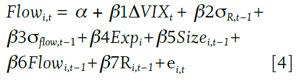
where, Flowi,t is monthly individual fund flow. ΔVIXt is the percentage change in VIX index levels, which is a measurement for investors looking for safe investments such as municipal bonds. δR,t−1 and δflow,t−1 are a fund’s monthly return volatility (standard deviation) and monthly flow volatility (standard deviation), respectively, calculated over a 12-month window. Expi,t is a fund’s expense ratio, Sizei,t−1 is the lagged total net asset value, and Flowi,t−1 is the lagged fund flow. These control variables are well documented in previous studies. For example, Rakowski (2010) found that flow is affected by flow volatility.
Table 5 presents the estimation result.6 The regression coefficients for VIX, the expense ratio, and fund size all had the expected sign and were significant. Results from the first pooled regression showed a significantly positive coefficient for the lagged fund raw return. However, the coefficient for the lagged excess return was insignificant when the market return was measured by either BC Index or ML Index returns. The same regression for each individual fund flow was evaluated.

As shown in Panel B of Table 5, only 15 funds exhibited a significantly positive coefficient for lagged raw returns, whereas the majority of the sample with 88 funds showed an insignificant regression coefficient. Under the BC Index as the benchmark, there were only six funds exhibiting a pattern consistent with return-chasing behavior. Similarly, under the ML Index as the benchmark, there were only five funds exhibiting a pattern consistent with return-chasing behavior. Thus, overall results suggest that HNW investors in municipal bond funds, unlike equity fund investors, do not exhibit a return-chasing behavioral pattern.
Market Indexes and Performance Evaluation
Figure 3 shows the difference in the number of funds outperforming each benchmark in each month. Not surprisingly, in every month, more funds outperformed the BC Index than outperformed the ML Index. In some months, the difference in the number of funds accounted for 90 percent of all funds in that month.
Additionally, the following hypothesis was tested: The selection of alternative indexes as the benchmark has no impact on the performance evaluation for individual funds.
Because the data frequency was monthly—not weekly—we tested this hypothesis by examining the effects of alternative benchmarks on a fund’s information ratio, which is defined as the ratio of a fund’s active return (excess return over the benchmark return, over the standard deviation of the active return). We calculated the information ratio for each fund for each year by using the average of the 12 monthly excess returns and its standard deviation. The information ratio is also called an appraisal ratio because it reflects a risk-adjusted return, reflecting a fund manager’s skills in taking more risk to generate higher returns.
Panel A of Table 6 presents the results. Using the BC Index as the benchmark, the average information ratio was significantly positive. In contrast, under the ML Index as the benchmark, the average information ratio was insignificant (p = .03). As indicated in the third column of Table 6, there was a significant difference in the information ratio for each fund between the two benchmarks. Using the BC Index as the benchmark, average fund managers do provide value from their active management, whereas there is no value from active management using the ML Index as the benchmark.
As shown in Panel B of Table 6, about 60 percent of the funds in the sample outperformed the BC Index, whereas only about 47 percent of the funds outperformed the ML Index. These results indicate that the two indexes, when used as the benchmark, have a significant bearing on the assessment of a fund’s performance evaluation. It is in each fund’s self-interest for a fund manager to choose the BC Index as their benchmark.
A fund manager may argue that investors do not lose anything from the selection of the BC Index as the benchmark, because a fund manager does not levy an incentive fee on investors; managers simply charge a fixed management fee based on AUM. However, such a defense is not valid to an investor paying attention to the information ratio or in cases where a fund reports beating the benchmark. Investors can certainly be harmed by the selection of an easy benchmark.
Implications for Planners and Money Managers
This study documents that returns from the ML Index are higher than those from the BC Index. It was also noted that individual fund returns are more closely related to ML Index returns. However, most long-term municipal bond mutual funds choose the BC Index as the benchmark. As a result, about 60 percent of funds are able to report outperforming the BC Index. However, using the ML Index as the benchmark, only about 47 percent of funds beat the benchmark.
The two indexes also tell a different story about the January effect. When returns from the BC Index are examined, evidence supports the January effect in the municipal bond market. However, when returns of the ML Index are tested, there is no evidence that returns are significantly higher in January than in other months.
Consistent with findings reported by Starks et al. (2006) for closed-end municipal bond fund returns, this study found that investors of municipal bond funds behave similarly in that they conduct tax-loss selling in December, but then rely on published fund performance for new investments.
The current use of market indexes has gone beyond the original purpose of reporting general performance of a market during a trading session. Market indexes are used as a benchmark to evaluate the performance of mutual funds and as the basis to create new investment vehicles such as exchange-traded funds, and index futures and options. These two functions make a market index increasingly important. Vendors regularly compete for the adoption of their own index by clients. It is no coincidence that firms such as CME Group, Dow Jones & Co., Barclays Capital, and Standard & Poor’s are forming joint ventures to create new indexes. As more indexes are created, investors need to pay attention to opportunistic selection by fund managers.
Under FINRA Regulatory Notice 09-35, FINRA encourages firms to review the overall adequacy and effectiveness of their current policies and procedures for municipal securities activities generally, particularly those relating to the disclosure of material information, the suitability of recommendations to retail customers, and the general supervision of their municipal securities activities. Clearly, the issue of conflicting indexes is not specifically addressed. However, FINRA appears to leave open to question the logic or motivation behind the selection of an index without disclosure of conflicting data, should that information be used by a client in their selection of a given bond fund. Given this and the differing results that the indexes represent, it would appear that, at minimum, financial planners should compare the two indexes. If a fund is selected using the BC Index, then the planner should disclose the ML Index ranking as well. This would precipitate a discussion on rankings and performance that would be to err on the side of full disclosure, which is always a safer route.
Endnotes
- The minimum market value for inclusion in the ML Index was $50 million before 2005. The data needed to compare the durations of the two indexes is not available.
- In the experience of the authors, advisers will use bond funds because either the firm that advises on or manages their funds uses mutual funds, or the advisers themselves prefer mutual funds for diversification and ease of management concentrating on financial planning instead of individual stock and bond selection and monitoring. Although some larger and more sophisticated advisory firms do in fact recommend individual bonds and stocks, smaller firms often do not. Further, tax loss selling is used to offset gains and 1099 filings from the mutual funds in an effort to remain tax neutral for clients.
- The returns RBC and RML were calculated with the logarithmic difference in the Barclays Capital Municipal Bond Index (BC) and the Merrill Lynch Municipal Securities Index (ML), respectively. Fund average R is a simple average monthly return of individual funds. R is individual fund returns for the 111 long-term national municipal bond mutual funds in the study. Index data spans from January 1980 to August 2011 for RBC and from January 1988 to August 2011 for RML. Data for individual funds vary depending on the inception dates, although all have the same cutoff date of August 2011. TNA Flowi is the fund flow. ∆VIX is the percentage change in the monthly VIX level. δR is fund return standard deviation over the previous 12 months. Expenses are expenses ratios.
- Panel A of Table 3 shows the seasonal pattern of the equally weighted average fund returns.
It also presents the results of including different market indexes in testing the average fund return seasonality. Ri is the return for individual long-tern national municipal bond mutual funds. Panel B reports the results from the following regression: Ri,t = Intercept + β1 January + β1 Rim,t + ei,t, where January is the dummy variable for the month of January. - Panel A of Table 4 presents monthly average fund flow. In Panel B, the dependent variable is a fund’s flow. In the December regression, the regression model is Flowi,t = Intercept + βLossi,t+ei,t, where the dependent variable is fund flow in December and the independent variable is a dummy variable that takes a value of one, if a fund’s cumulative returns (Ri,cu) from January to November is negative, and zero otherwise. In the January regression, the model is Flowi,t = Intercept + βLossi,t+ei,t, where the dependent variable is fund flow in January.
- Panel A of Table 5 presents results from a pooled regression. Panel B presents the individual fund regression results. The dependent variable is a fund’s flow. In model 1, Ri,t−1 is a fund’s lagged raw return. In the BC Index model, we replaced a fund’s raw return with the excess return over the BC Index return. Similarly, in the ML Index model, we used the excess return over the ML Index return. ∆VIXt is the monthly percentage change in the level of CME’s VIX index. δR,i and δflow,t−1 are the standard deviation of individual fund raw returns and flow over the past 12 months, respectively. Expi,t is the expense ratio. Sizei,t−1 is a fund’s lagged total net asset value.
References
- Ackermann, Carl, Richard McEnally, and David Ravenscraft. 1999. “The Performance of Hedge Funds: Risk, Return, and Incentives.” The Journal of Finance 54 (3): 833–874.
- Ang, Andrew, and Richard Carleton Green. 2011. “Lowering Borrowing Costs for States and Municipalities Through CommonMuni.” Hamilton Project, Brookings Discussion Paper.
- Berk, Jonathan B., and Richard C. Green. 2004. “Mutual Fund Flows and Performance in Rational Markets.” Journal of Political Economy 112 (6) 1269–1295.
- Bollen, Nicolas P.B., and Jeffrey A. Busse. 2004. “Short-Term Persistence in Mutual Fund Performance.” The Review of Financial Studies 18 (2): 569–597.
- Chen, Haiwei, Jim Estes, and Thanh Ngo. 2011. “Tax Calendar Effects in the Municipal Bond Market: Tax-Loss Selling and Cherry Picking by Investors and Market Timing by Fund Managers.” Financial Review 46 (4): 703–721.
- Chen, Hsiu-lang, and George G. Pennacchi. 2009. “Does Prior Performance Affect a Mutual Fund’s Choice of Risk? Theory and Further Empirical Evidence.” Journal of Financial and Quantitative Analysis 44 (4): 745–775.
- Chevalier, Judith A., and Glenn D. Ellison. 1995. “Risk Taking by Mutual Funds as a Response to Incentives.” National Bureau of Economic Research Working Paper No. w5234.
- Edelen, Roger M. 1999. “Investor Flows and the Assessed Performance of Open-End Mutual Funds.” Journal of Financial Economics 53 (3): 439–466.
- Fant, Franklin L. 1999. “Investment Behavior of Mutual Fund Shareholders: The Evidence from Aggregate Fund Flows.” Journal of Financial Markets 2 (4): 391–402.
- Grinblatt, Mark, and Sheridan Titman. 1994. “A Study of Monthly Mutual Fund Returns and Performance Evaluation Techniques.” Journal of Financial and Quantitative Analysis 29 (3): 419–444.
- Ippolito, Richard A. 1992. “Consumer Reaction to Measures of Poor Quality: Evidence from the Mutual Fund Industry.” Journal of Law & Economics 35 (1): 45–70.
- Jakob, Keith, and Bruce A. Costa. 2011. “Are Mutual Fund Managers Selecting the Right Benchmark Index?” Financial Services Review 20 (2): 129–140.
- Lee, Charles, Andrei Shleifer, and Richard H. Thaler. 1991. “Investor Sentiment and the Closed-End Fund Puzzle.” The Journal of Finance 46 (1): 75–109.
- Lehmann, Bruce N., and David M. Modest. 1987. “Mutual Fund Performance Evaluation: A Comparison of Benchmarks and Benchmark Comparisons.” The Journal of Finance 42 (2): 233–265.
- Lynch, Anthony W., and David K. Musto. 2003. “How Investors Interpret Past Fund Returns.” The Journal of Finance 58 (5): 2033–2058.
- Poterba, James M., and Scott J. Weisbenner. 2001. “Capital Gains Tax Rules, Tax-Loss Trading, and Turn-of-the-Year Returns.” The Journal of Finance 56 (1): 353–368.
- Rakowski, David. 2010. “Fund Flows Volatility and Performance.” Journal of Financial and Quantitative Analysis 45 (1): 223–237.
- Robbins, Mark D., and Bill Simonsen. 2013. “Municipal Bond New Issue Transaction Costs.” Public Budgeting & Finance 33 (1): 1–24.
- Sensoy, Berk A. 2009. “Performance Evaluation and Self-Designated Benchmark Indexes in the Mutual Fund Industry.” Journal of Financial Economics 92 (1): 25–39.
- Sirri, Erik R., and Peter Tufano. 1998. “Costly Search and Mutual Fund Flows.” The Journal of Finance 53 (5): 1589–1622.
- Starks, Laura T., Li Yong, and Lu Zheng. 2006. “Tax-Loss Selling and the January Effect: Evidence from Municipal Bond Closed-End Funds.” The Journal of Finance 61 (6): 3049–3067.
Citation
Chen, Haiwei, Jim Estes, and Daniel Jubinski. “Our Benchmark Is Better Than Your Benchmark: The Municipal Bond Market.” Journal of Financial Planning 27 (7): 50–59.