Journal of Financial Planning: January 2021
Executive Summary
- Reverse mortgages can facilitate larger allocations to equities as a percentage of net worth. By owning more equities for more time, retirees may be able to enhance their probability of cashflow survival and estate expectations.
- Specifying the equity allocation as a percentage of net worth leads to strategies that coordinate account allocations with the debt decision. This allows the retiree to avoid maintaining a negative interest rate spread.
- Unless the retiree intends to leave her tax-deferred account to charity, it is important to adjust the estate value to adjust for the deferred tax. Because charities do not need to pay income tax on tax-deferred assets bequeathed to them, borrowing rather than using IRA distributions for expenses may significantly enhance the value of the estate through the reduction of taxes. However, if the intended heirs have a higher tax rate than the retiree, this may be destructive.
Charles Fox, CFA, is a partner and financial adviser at Integrity Wealth Partners in Walnut Creek, CA. He graduated from Princeton University with an undergraduate degree in operations research and financial engineering.
NOTE: Please click on the Tables and Figures below to open PDF versions of the images.
JOIN THE DISCUSSION: Discuss this article with fellow FPA Members through FPA's Knowledge Circles.
According to the 2013 Survey of Consumer Finances, the primary residence represents over half of total wealth for most U.S. households over age 65 (Davidoff, Gerhard, and Post 2016). As a result, converting home equity into cashflow is often an important part of retiree financial plans. Many people feel an emotional attachment to their homes and do not wish to sell or leave.
Home Equity Conversion Mortgages (HECM) are a collection of loan products that generally allow retirees to defer repayment until permanently leaving the home. In addition to residing in the home, the borrower is required to maintain the home, pay property taxes, and pay homeowners insurance premiums. Since 2013, the Department of Housing and Urban Development has imposed regulations intended to prevent the origination of HECM reverse mortgages that are likely to lead to a default on these obligations (Pfau 2015).
As of 2017, only about 0.2 percent of homeowners 65 and older had an active HECM. Misunderstandings and incomplete knowledge of reverse mortgages have been cited as contributing factors to the low uptake rate (Davidoff, Gerhard, and Post 2016 as cited in Cackley et al. 2019). Pfau (2015) noted that many advisers maintain a dismal view of reverse mortgages and implored them to revisit their outdated thinking in light of supportive academic research. This article will review, extend, and reframe this academic research, and will review the importance of income tax effects of inherited accounts on the results presented in prior work.
Some of the prior simulation studies have treated deferred tax retirement accounts and after-tax assets equally when calculating estate values. This may be appropriate when the retiree’s beneficiary is a charity. For retirees who wish to leave their estate to children or other individuals, a dollar of tax-deferred assets is not fungible with a dollar of mortgage debt.
This article will extend the reverse mortgage simulation literature by including life after the sale or foreclosure of the primary residence. If the retiree is unable to fund her living expenses, including property tax, she sells the home or experiences foreclosure. After leaving the primary residence, a rent expense is added to her living expenses. This allows for complete use of the home’s equity in determining cashflow survival.
Finally, prior reverse mortgage simulations have specified the equity allocation as a percentage of the investment account. Under this specification, a simulated retiree with more debt owned more equities than another retiree with the same net worth and equity allocation setting. This article will reframe prior analysis by specifying the equity allocation as a percentage of the retiree’s net financial worth. Not only does this cause two debt strategies with the same equity allocation setting and net worth to own the same amount of equities, it also has the positive side effect of leading to strategies that avoid using debt while owning lower yielding fixed income investments. The avoidance of negative interest rate spread leads to higher simulated cashflow survival rates and financial net worth than strategies that do not include this feature.
Literature Review
Sacks and Sacks (2012) found that active use of a reverse mortgage credit line throughout retirement significantly increased cashflow survival rates and residual net worth relative to waiting to establish a line of credit upon exhaustion of the investment portfolio.
Wagner (2013) advanced this research by extending the analysis to include term loans. The article found that the increase in portfolio value due to reduced withdrawals was often greater than the interest expense associated with a reverse mortgage. It also demonstrated that if the 10-year rate at the beginning of retirement is higher than the expected average short-term rate, opening a line of credit at the beginning of retirement generally allows a retiree to borrow more than if she waits until the exhaustion of the investment portfolio to open the line of credit.
Pfeiffer et al. (2014) found, and Pfau (2016) confirmed, that opening a line of credit early in retirement—but waiting to use it until the retirement portfolio is exhausted—increases the probability of cashflow survival. The article also demonstrated a tradeoff between a larger expected estate if the retiree borrows early versus a lower probability of cashflow failure if the retiree waits to borrow.
Pfau (2019) argued that reverse mortgages can enhance the final estate, despite high costs due to the preservation of retirement account assets. This was illustrated through a single historical time series rather than simulation.
Cackley et al. (2019) found that defaults as a percentage of HECM terminations grew from 2 percent in 2014 to 18 percent in 2018. They also noted that due to reporting weaknesses by the Federal Housing Administration (FHA), the termination reasons for about 30 percent of HECMs are unknown. The report does not break down the defaults by origination date. Without disaggregated data and complete termination reason data, it is unclear whether loans originated after the 2013 reforms have had better outcomes than their predecessors. As a result, financial planners rely on theoretical studies to evaluate the relative benefits and costs of reverse mortgages.
One of the appeals of a reverse mortgage is that because it is a loan, the cashflow is received tax-free. Strategies were developed to facilitate the deduction of reverse mortgage interest payments prior to the Tax Cuts and Jobs Act of 2017 (TCJA) (Sacks, et al. 2016, as cited in Kitces 2017). However, the TCJA disallowed the deduction of mortgage interest for non-acquisition purposes (Kitces 2018).
Blanchett and Straehl (2015) demonstrated the importance of a full-balance sheet approach to portfolio management. They integrated human capital, housing wealth, pensions, and investment accounts into portfolio optimization. Their analysis included a mortgage, but not a reverse mortgage.
Analysis
The analysis begins with an examination of the historical back test comparing the use and non-use of a reverse mortgage detailed in Pfau (2019). After describing alternative approaches in the context of the historical back test, a simulation analysis is presented to test the intuition developed by the back test.
Back test. The following analysis reviews the impact of including the deferred tax liability for the inherited retirement account would have had if it were included in the back test found in Pfau (2019). A debt-free strategy that attempts to own the same amount of equities as the reverse mortgage strategy is added to the comparison. Finally, a strategy that opens a line of credit but waits to access it until after all fixed income securities are sold is also added.
After-tax legacy value. The appropriate calculation of a retiree’s legacy value is a function of who (or what) will be receiving the estate. If a retiree intends to leave her estate to charity, no adjustment is required to the value of tax-deferred assets because the charity will not need to pay income tax. However, many retirees intend to leave their estates to children or other individuals. For these retirees, it is appropriate to adjust the value of the retirement account to reflect the income taxes the heirs will need to pay upon receiving disbursements from the account (Kitces 2015, Pfau 2018).
A retiree needs to distribute $1/(1 – TAX_RATE) from tax-deferred accounts for each dollar of expenses she needs to cover. In contrast, if she uses debt, she only needs to borrow one dollar per dollar of expenses. As a result, if a retiree intends to make charitable bequests, debt can be a powerful tool to preserve tax-deferred assets, which can pass to the charity tax-free. If her heirs are in the same tax bracket she is, using debt instead of a distribution has the immediate effect of making the potential gross estate larger, but leaves the net value unchanged.
It is unclear how common the assumption of zero tax adjustment for tax deferred accounts has been in the reverse-mortgage literature. For example, Wagner (2013) does not mention an adjustment but does not explicitly state none was made. Sacks and Sacks (2012) do not mention an adjustment, but also do not seem to have used larger distributions than debt draws for the same expense. If this is the case, the account was treated like a Roth, which would not need an adjustment for cross strategy comparison.
Pfau (2019) argued that the effects of a reverse mortgage on a retiree’s final estate are often misunderstood. In support of this claim, a detailed back test was provided, which demonstrated that the retirement account growth permitted by using debt instead of a distribution for one year’s living expenses more than offset the costs associated with the debt, leading to a larger estate. The article included tables illustrating the progression of the hypothetical retiree’s expenses and balance sheet. Because of the detailed table, it can be clearly understood that no tax adjustment was made to the legacy value in this analysis, which is appropriate if the IRA is left to charity.
Starting Conditions
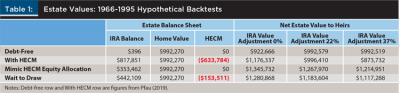
In Pfau (2019), a hypothetical person retired in 1966 at age 65 with an IRA and $200,000 home. She faced a 22 percent flat income tax rate. Her total non-tax expenses in the first year were $31,502.65 and her expenses grew with inflation.
The analysis compared two strategies. Both strategies allocated 50 percent of the IRA balance to the S&P 500 and 50 percent to intermediate-term government bonds. In the first strategy, the retiree did not access her home equity. In the second, she paid $13,721 of fees to draw $51,309 at the beginning of 1975, when she was 74. The origination fees were added to the amount borrowed. The balance grew each year at the one-year treasury rate, plus 3 percent.
Pfau (2019) found that using an HECM resulted in a larger final net legacy value, defined as IRA balance plus home value minus loan balance. The results computed in Pfau (2019) are in the first two rows of Table 1. If she bequeathed her IRA to charity, the reverse mortgage added $183,671 of value relative to the debt-free strategy. If the IRA’s value is adjusted by her tax rate, 22 percent, the advantage of the reverse mortgage strategy over the debt-free strategy drops to less than $4,000. If her heir is in a higher marginal tax bracket because of income from other sources, a larger adjustment would be justified. In this case, the debt-free strategy would have produced a larger tax-adjusted value than the reverse mortgage strategy.
Risk
If a retiree uses debt to maintain an investment portfolio, her net worth will be more volatile than if she remains debt free and uses the same investment account allocations. Two investment accounts with the same percentage allocation will have the same percentage gains and losses, but the larger account will have larger dollar gains and losses.
In Pfau (2019), the hypothetical retiree used a 50 percent allocation to equities in her IRA for both the reverse mortgage and the debt-free strategies. At age 90, this corresponded to 16 percent of her tax-adjusted net worth allocated to equities for the debt-free strategy, but 30 percent for the reverse mortgage strategy. Yet, as shown previously, if the heirs are assumed to have the same effective income tax rate on distributions as her, the tax-adjusted estate value was roughly the same, with and without the reverse mortgage.
To test the importance of the equity allocation, a third strategy was tested. Each year, the hypothetical retiree invested the same dollar amount in equities as in the reverse mortgage strategy, up to the full balance of the IRA. As shown in the third row of Table 1, this resulted in a larger final estate than the reverse mortgage strategy, even without adjusting the IRA balance to reflect the deferred tax liability. This suggests that the reverse mortgage has served as an expensive source of courage to own more equities in some simulations.
Some of the increased courage may be justified. When opened, a line of credit provides a source of credit that is unaffected by changes in the home’s value. This may be a source of comfort for those who choose to open one. In a prior simulation study, opening a line of credit but waiting to utilize it until the retirement account was depleted was found to have the highest survival rate of all strategies tested, highlighting its risk-reducing power (Pfau 2016).
Because the retirement account was not fully depleted in this back test, opening a line of credit to only be utilized after depletion would not have increased the final estate. However, the debt-free strategy, in the third row of Table 1, which attempted to own the same amount of equities as the reverse mortgage strategy, was unable to do so in the final year because the IRA was smaller than the target equity allocation. A fourth strategy was evaluated, which opened the line of credit early in retirement but waited to borrow until paying for living expenses; using an IRA distribution would cause the IRA value to fall below the target equity ownership amount. As shown in the fourth row of Table 1, this strategy produces a larger estate than borrowing early in retirement but a smaller estate than not borrowing.
Negative Interest Spread
It is usually suboptimal to lend at a lower rate than the cost of funds. The average annual cost of borrowing using the HECM in Pfau (2019) was 11.5 percent. During the time period the loan was used, the average fixed-income return was 9.8 percent. By reducing the allocation to fixed income rather than simultaneously maintaining the fixed-income allocation while borrowing, the last two strategies were able to avoid this negative spread. Because the hypothetical HECM’s annual costs were one-year treasuries plus 3 percent, significant returns attributable to a term premium, decline in long term rates, credit, or other sources would have been required for a fixed income investment to outperform the cost of debt. The inclusion of investment management fees would have made this negative spread even more severe.
Although the avoidance of a negative interest spread allows the third and fourth strategies to outperform the second strategy, it would be impractical for a retiree to choose an equity allocation equal to the allocation they would have used following a different financial plan. Instead, a full-balance sheet approach to the equity allocation may be used. Aside from origination costs, a retiree’s net worth does not change the moment money is borrowed. The proceeds received equal the debt. As a result, specifying the allocation as a percentage of net worth prevents borrowing from triggering an immediate and significant increase to the dollar amount allocated to equities, creating consistency across strategies.
Simulation
Assumptions. To test the generalizability of the findings from the back test, 2,000 sets of five random variates per year were generated. The same 2,000 sets were applied to each strategy.
The initial retiree age, home value, and tax-deferred retirement account value were 63, $450,000 and $800,000 respectively. The retiree’s monthly expenses for the first year were $2,583. A flat tax rate of 1 – 2583/4000, or 35.4 percent was assumed. Required minimum distributions were not considered and the retiree had no other sources of income. All of the assumptions in this paragraph were previously used in Wagner (2013).
The market data simulation was calibrated using a mixture of forward-looking market data as of August 31, 2020, and annual historical data from the beginning of 1987 through the end of 2019. The first year of data for the Case-Shiller U.S. National Index on FRED was 1987 (FRED is the economic database published by the Federal Reserve Bank of St. Louis). Inflation was simulated using an average of 1.8 percent, the difference between the 10-year nominal treasury yield and 10-year real yield on August 31, 2020.
The 10-year treasury rate as of August 31, 2020, 0.72 percent, was used as the initial 10-year rate (United States Treasury 2020). Changes in the 10-year rate were simulated from a normal distribution with zero mean and 1.06 percent standard deviation. The return to fixed income was calculated using the prior year’s yield and the updated yield. Pfau (2016) also generated bond returns by simulating a change in yield. Because it is unknown how negative interest rates may go, no floor was imposed on interest rates. The impact of the most extreme interest rate paths on the analysis was mitigated by using the median rather than the mean for legacy value analysis.
The initial one-year treasury rate was 0.12 percent, the rate as of August 31, 2020. For the first 10 years, the change in the one-year rate was simulated with an average increase of 0.12 percent. After the tenth year, the average change was set to zero. This creates consistency with the initial 10-year rate. The simulations in Pfau (2016) also used a positive drift term when simulating short-term rates.
The equity risk premium was simulated with an average of 8.67 percent and a standard deviation of 16.48 percent, consistent with the annual returns from 1987 through 2019 (Morningstar 2020). Equity returns were simulated as the sum of the one-year rate and the equity risk premium.
Home appreciation was simulated from a normal distribution with annualized average of 3.08 percent. This was calibrated as the sum of the forward-looking inflation assumption and the average real appreciation of the Case-Shiller U.S. National Index from its inception in 1987 through 2019. The simulated standard deviation was 11.96 percent, the standard deviation of the S&P/Case-Shiller San Francisco region for the same time period (S&P 2020). No additional volatility was added to account for the idiosyncratic risk of the house. The correlation matrix was calculated using annual data from 1987 through 2019.
The annual mortgage insurance premium (MIP) for strategies that utilized an HECM was 0.5 percent. Lender’s margin was assumed to be 2.25 percent. The retiree’s initial principal limit was calculated using an expected rate of 3 percent and the October 2017 Principal Limit Factor Tables. The cost of debt was not allowed to increase or decrease more than 5 percent after origination. The resulting initial limit was $238,500 (53 percent of the home value). The origination fees, closing costs, and upfront mortgage insurance premium were assumed to be $6,000, $2,500, and $9,000, respectively, for a total upfront cost of $17,500.
The retiree was assumed to rent a comparable home if homeownership ceased. The net increase in expenses due to rent, less the costs of homeownership, was assumed to be one-fifteenth of the home value. Six percent transaction costs were assumed on any sale. Capital gains taxes were assumed to be 15 percent of the net sale price above $700,000—the initial home value, plus the $250,000 capital gains exclusion for single taxpayers who satisfy the residency requirement. If homeownership ceased due to foreclosure, the mortgage debt was forgiven, and capital gains tax was assessed using the loan balance as the sales price.
The net proceeds from any sale were invested into a non-retirement taxable investment account. Fixed income returns in this account were taxed at the ordinary income tax rate. Equity returns were taxed annually at the capital gains rate. No additional tax was assumed on withdrawal. If all of the retiree’s resources were exhausted, shortfall was tabulated without interest.
Retirement Cashflow Strategies Evaluated
Retirement strategies were simulated using both an equity allocation specified as a percentage of account value and as a percentage of tax-adjusted net worth.
Five strategies were simulated under both specifications.
Debt free. The retiree used distributions from her IRA to pay for her living expenses. If the IRA was depleted, she sold her home.
Open, use upon depletion. The retiree opened a line of credit at the beginning of her retirement. She paid the origination fees using her IRA. She funded her living expenses using distributions from the IRA until it was depleted. Next, she borrowed from her line of credit to pay for her living expenses. This strategy is similar to the “Use Home Equity Last” strategy used in Pfau (2016). Once she exhausted her line of credit, she sold her home or allowed it to be foreclosed.
Open upon depletion. The retiree used distributions from her IRA to pay for her living expenses until it was exhausted. Next, she opened a line of credit. The origination fees were paid using the line of credit. The origination fees and maximum eligible amount were assumed to grow with inflation. Her maximum amount to borrow was computed using the home price, 10-year interest rate, and her age at the time of opening. Once the line of credit was fully utilized, she sold her home or allowed it to be foreclosed. This strategy was similar to the “Home Equity as Last Resort” strategy in Pfau (2016).
Term loan. The retiree received fixed payments of $2,583 per month for 107 months from an HECM loan. This covered all expenses for the first year. IRA distributions were used to pay living expenses in excess of the fixed draws. In the rare paths with deflation, the amount borrowed above living expenses was invested into the taxable account and used toward expenses in the following year. This strategy was similar to the “Term Loan First” strategy in Wagner (2013).
Sacks and Sacks coordinated. For this strategy, the retiree opened a line of credit at the beginning of retirement and paid the origination costs and her first year living expenses using her IRA. In the second and all subsequent years, if the IRA had a positive return in the prior year or if the home equity line was used to capacity, the retiree used a distribution from the IRA to fund her living expenses. If the prior year IRA return was negative or if her IRA was exhausted, she drew from the home equity line. If the home equity line was fully utilized and her IRA was exhausted, she sold the home or experienced foreclosure. This was intended to implement the coordinated strategy in Sacks and Sacks (2012), which avoids depleting the IRA after losses.
Two additional strategies were evaluated in the version of the simulation in which the equity allocation was specified as a percentage of the tax-adjusted net worth.
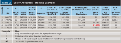
Open, use to maintain risk. The retiree opened a line of credit at the beginning of her retirement. She paid the origination fees using her IRA. She paid for her living expenses using her IRA until her IRA was too small to meet her target equities allocation. Once this occurred, she funded her living costs using the line of credit. If positive equity returns or a decline in the home price caused her IRA value to subsequently exceed the target equity allocation—and her home had positive equity—she resumed using IRA distributions to pay for her living expenses. If the IRA was large enough to exceed the equity target after paying for her living expenses, she also used a distribution from her IRA to reduce her loan balance. Once she exhausted her line of credit and fully depleted her IRA, she sold her home or allowed it to be foreclosed.
Open once needed to maintain risk. The retiree did not open a line of credit at the beginning of retirement. She retiree paid her living expenses using her IRA until her IRA was too small to meet her target equities allocation. Once this occurred, she opened a line of credit and paid the origination costs with debt. This strategy is otherwise the same as the preceding one.
To help explain these final two strategies, Table 2 illustrates their decisions in a few hypothetical scenarios. Table 2 assumes the line of credit has been established. Once the line of credit was opened, the final two strategies behaved identically.
Results
Account percentage specification. The first set of results were calculated using equity allocations specified as a percentage of account balance. These results serve primarily as a useful comparison to the existing literature.
Figure 1 shows the rate of homeownership after 30 years. This is equivalent to the survival metrics from prior studies, which did not include the possibility of cashflow survival as a renter.
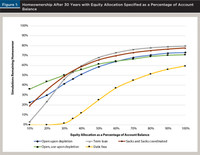
Consistent with the results in Pfau (2016), considering home equity as a last resort once the retirement account was depleted produced the lowest long-term homeownership rate of all reverse mortgage strategies for equity allocations between 30 and 60 percent.
For the three strategies that originated the reverse mortgage at the beginning of retirement, there is a clear crossing point at an equity allocation of 35 percent. At an equity allocation of 35 percent, the expected return of the IRA was roughly equal to the growth rate of the line of credit. As a result, higher equity allocations favored the term loan that borrows early, and lower equity allocations favored waiting to use debt until the IRA was depleted. The Sacks and Sacks Coordinated strategy, which borrows sporadically throughout the life of the IRA, was a middle ground. Across all strategies, the survival rates were significantly lower than those found in Wagner (2013). This is primarily a reflection of the fall in interest rates since 2013, which reduced expected return assumption for fixed income investments. The 2017 update to the principal limit factor tables also caused a reduction in the amounts available to borrow for low expected rates.
Figure 2 displays the cashflow survivorship after 30 years. The debt-free strategy shows the biggest gap between survival and homeownership. The strategy had more home equity upon departure from the home than the other strategies. However, the debt-free strategy still had a lower cashflow survival than the reverse mortgage strategies. For the remaining strategies, the increase in survival due to extending the model to include the post-homeownership period was fairly similar: ranging from about 10 percent for smaller equity allocations to about 4 percent for the highest equity allocations.
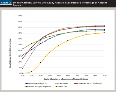
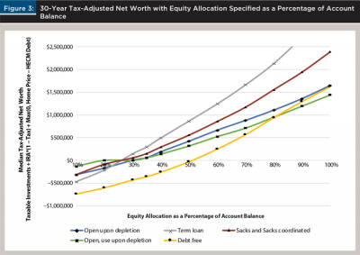
Figure 3 illustrates the median tax-adjusted net worth for each strategy. Simply, a larger allocation to equities—whether through direct specification, leverage, or both—produced a larger median net worth. Similarly, for most equity allocations, the avoidance of origination costs led to outperformance for the open upon IRA depletion strategy relative to the open but wait to use until depleted strategy.
Tax-adjusted net worth percentage specification. This set of results was calculated using equity allocations specified as a percentage of the retiree’s tax-adjusted net worth. With the allocation specified as a percentage of tax-adjusted net worth, the decision to borrow or not borrow can be coordinated with the rest of the balance sheet. These results show the value created by using this coordination to avoid negative interest rate spread.
Figure 4 shows the cashflow survival for all strategies tested under this specification. The results for the term-loan strategy were poor compared to its results in Figure 2 because borrowing early resulted in more negative interest rate spread exposure instead of more equity exposure with this specification. The Sacks and Sacks coordinated strategy also occasionally borrowed while the IRA still owned fixed income, but far less often than the term-loan strategy did. As a result, its survival rate was much higher than the term-loan strategy’s survival rate. The strategy that opens the line of credit at the beginning of retirement but does not begin to borrow until all fixed income is sold, thus, completely avoiding the negative interest rate spread, had the highest survival rate for all equity allocations under this specification.
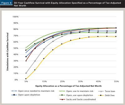
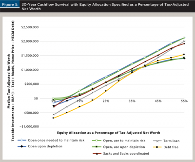
Figure 5 shows the median tax-adjusted net worth for all strategies tested under this specification. The term loan strategy generally underperformed other reverse mortgage strategies. With fairly high equity allocations, the Sacks and Sacks coordinated strategy produced a higher net worth than strategies that did not borrow before the depletion of the IRA. The strategies that avoided simultaneously borrowing and owning fixed income dominated those that did not. Waiting to open a line of credit until the IRA balance was too small to reach the risk target produced a slightly larger median net worth for most allocations than opening the line of credit at the beginning of retirement.
Limitations and Potential Extensions
The simulation model in this paper omitted important features of a retiree’s real experience.
This research only examined the retiree’s net worth and cashflow survival over a fixed time horizon. It could be extended by including random death and health-induced relocation to a nursing home. It also omitted investment management fees, required minimum distributions, and progressive income taxation.
More sophisticated capital markets assumptions could be used. For example, a floor could be imposed on interest rates. The inclusion of parameter ambiguity, rather than simulating all paths from the same distribution, could also be a valuable contribution.
The retiree’s strategies could be extended to include duration immunization. If the fixed-income investment is sufficiently correlated to the expense liabilities or negatively correlated with the equity risk premium, it may be worthwhile to use leverage, even at a negative interest rate spread. If this is the case, leveraged closed-end funds and derivatives could be explored as alternatives to reverse mortgages for maintaining duration exposure. This exploration could be especially valuable for retirees whose heirs are in a high tax bracket.
Conclusions
HECM loans are a powerful tool that can be especially valuable for retirees with tax-deferred assets and a desire to leave those assets to charity. They can also create value when used to fund investment in assets with a higher expected return than the cost of the debt. However, retirees with conservative account allocations and HECM debt outstanding may benefit from selling low-yielding fixed-income investments to pay off debt. By transitioning to a strategy that avoids a negative interest rate spread, retirees may be able to enhance both their cashflow survival rates and their expected estates. Reframing risk conversations from percentages of account value to a full balance sheet approach is essential for this transition. Financial planners can present their clients forecasted balance sheets with and without HECM loans to identify the potential for a negative interest rate spread and discuss the desired equity allocation relative to the full balance sheet.
References
Blanchett, David M., and Philip U. Straehl. 2015. “No Portfolio is an Island.” Financial Analysts Journal 71 (3): 15–33.
Cackley, Alicia Puente et al. 2019. “Reverse Mortgages FHA Needs to Improve Monitoring and Oversight of Loan Outcomes and Servicing.” U.S. Government Accountability Office. Available at www.gao.gov/assets/710/701676.pdf.
Davidoff, Thomas, Patrick Gerhard, and Thomas Post. 2016. “Reverse Mortgages: What Homeowners (Don’t) Know and How it Matters.” Available at papers.ssrn.com/sol3/papers.cfm?abstract_id=2651032.
Kitces, Michael. 2018. “Acquisition And Home Equity Mortgage Interest Tax Deductibility After TCJA.” Available at www.kitces.com/blog/tcja-home-mortgage-interest-tax-deduction-for-acquisition-indebtedness-vs-home-equity-heloc/.
Kitces, Michael. 2017. “The Taxation of Reverse Mortgage Loan Proceeds and Interest Payments.” Available at www.kitces.com/blog/hecm-reverse-mortgage-interest-deduction-insurance-premiums-and-real-estate-taxes/.
Kitces, Michael. 2015. “When A Roth IRA May Actually Be A Terrible Asset to Inherit.” Available at www.kitces.com/blog/when-a-roth-ira-may-actually-be-a-terrible-asset-to-inherit/.
Morningstar. 2020. “Stocks, Bonds, Bills, and Inflation (SBBI) Data.” CFA Institute. Available at www.cfainstitute.org/en/research/foundation/sbbi.
Pfau, Wade D. 2015. “Advisors Need a Fresh Look at Reverse Mortgages.” Advisor Perspectives. Available at www.advisorperspectives.com/articles/2015/12/01/advisors-need-a-fresh-look-at-reverse-mortgages.
Pfau, Wade D. 2019. “What the Critics Get Wrong About Reverse Mortgages.” Advisor Perspectives, Available at www.advisorperspectives.com/articles/2019/04/15/what-the-critics-get-wrong-about-reverse-mortgages.
Pfau, Wade D. 2016. “Incorporating Home Equity into a Retirement Income Strategy.” Journal of Financial Planning 29 (4): 41-49.
Pfau, Wade D. 2018. Reverse Mortgages: How to Use Reverse Mortgages to Secure Your Retirement. 2nd. McLean, Va.: Retirement Researcher Media.
Pfeiffer, Shaun, C. Angus Schaal, and John Salter. 2014. “HECM Reverse Mortgages: Now or Last Resort.” Journal of Financial Planning 27 (5): 44–51.
S&P Dow Jones Indices LLC. 2020. S&P/Case-Shiller U.S. National Home Price Index. FRED, Federal Reserve Bank of St. Louis. Available at fred.stlouisfed.org/series/CSUSHPISA.
Sacks, Barry H., and Stephen R. Sacks. 2012. “Reversing the Conventional Wisdom: Using Home Equity to Supplement Retirement Income.” Journal of Financial Planning 25 (2): 43–52.
Sacks, Barry H., Nicholas Maningas Sr., Stephen R. Sacks, and Francis Vitagliano. 2016. “Recovering a Lost Deduction.” Journal of Taxation April: 157–169.
United States Treasury. 2020. Available at www.treasury.gov/resource-center/data-chart-center/interest-rates/Pages/TextView.aspx?data=yield.
Wagner, Gerald C. 2013. “The 6.0 Percent Rule.” Journal of Financial Planning 26 (12): 46–54.
Citation
Fox, Charles. 2021. “No Debt is an Island: Exploring Strategies with Reverse Mortgages.” Journal of Financial Planning 34 (1): 60–70.