Journal of Financial Planning: January 2020
Executive Summary
- Conventional wisdom holds that during a bear market, holding is good and rebalancing is better. This paper examines the effects of rebalancing to a more aggressive target than originally intended—specifically, rebalancing a 50/50 stock/bond portfolio to a 60/40 ratio at the point a decline in stocks reaches 20 percent, rather than rebalancing back to 50/50 or not rebalancing at all. During severe bear markets, three other rebalancing strategies were also considered.
- For the various rebalancing strategies, results include the time it took for the portfolio to recover; the value of rebalanced portfolios as of the date a never-rebalanced portfolio recovered on its own; and the portfolio values three years after the start of a bear market.
- Findings indicate that rebalancing to either the original 50/50 target, or a more aggressive 60/40 once stocks decline 20 percent, generally provided minimal improvements in the metrics examined, versus not rebalancing at all. Rebalancing activity during a more severe decline of 40 percent provided more improvements, but many clients may not be willing to implement the most aggressive approaches examined.
- For clients with flexibility about their choice of stock-to-bond ratio and a suitable temperament, aggressive rebalancing may be appealing. However, the improvements observed were generally so modest, manipulating portfolio structure through aggressive rebalancing may not impact goal achievement as much as other actions, such as recommending clients save more, spend less,
manage taxation, or work longer.
Dan Moisand, CFP®, is a fee-only financial adviser in the Melbourne, Fla. office of Moisand Fitzgerald Tamayo, LLC, regarded by many as one of America’s top financial advisers for retirees and near retirees. He is a past national president of FPA and has been featured as one of America’s top financial planners by at least 10 financial planning publications.
Mike Salmon, CFP®, EA, is an adviser who has been with Moisand Fitzgerald Tamayo, LLC since 2007. His expertise lies in the areas of retirement and tax planning. He assists in tax preparation of individual and corporate tax returns as well as year-end tax projections. Salmon was recognized by Financial Advisor magazine as a 2018 “10 Young Advisors to Watch.”
JOIN THE DISCUSSION: Discuss this article with fellow FPA Members through FPA's Knowledge Circles.
From the first day one considers in earnest the subject of investing, it is clear that selling out of stocks after a significant decline is almost universally described as a bad move for long-term investors. Even if someone gets back into the market at a lower price point after exiting, that success encourages further speculations of what the market may do next, resulting in additional bets for bigger and bigger sums of money until being wrong costs dearly.
“Be fearful when others are greedy and greedy when others are fearful,”1 is a well-known and well-regarded piece of investing wisdom attributable to Warren Buffett; but alas, it is often not followed.
Safe withdrawal rate and portfolio sustainability studies typically assume that portfolios are rebalanced, usually annually, regardless of market behavior. For diversified portfolios, during a bear market, the conventional wisdom seems to be that selling is bad, holding is okay, and rebalancing is better.
Review of Rebalancing
Rebalancing requires buying an asset class when that asset class lags others in the portfolio. Rebalancing leads to buying equities during bear markets. Rebalancing restores the risk/reward profile of the portfolio and can enable the portfolio to recoup losses faster than it would have if no rebalancing was performed.
For example, consider a 50/50 allocation for $200,000 split $100,000 each between “A,” a hypothetical stable bond fund, and “B,” a hypothetical stock fund, where A earns 4 percent while B loses 20 percent. As shown in Panel A of Table 1, the total portfolio is down 8 percent with a value of $184,000 (A = $104,000 and B = $80,000).
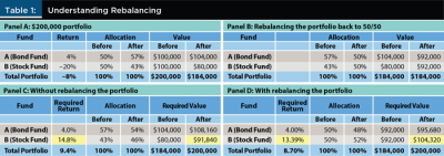
The portfolio now sports a 57 percent (A) to 43 percent (B) mix. It is over-exposed to the risks and potential return of A, and underexposed to the risks and potential return of B. To rebalance back to 50/50, $12,000 of A is sold to buy $12,000 of B, leaving $92,000 in each fund (see Panel B of Table 1).
The investor has lost $16,000 and just bought $12,000 more of the very thing that caused the loss. Therefore, at this point, how rebalancing provides risk control and a defense against emotional tactical decision-making may not be obvious to the client. (The emotional aspects of rebalancing will be discussed later.)
Without rebalancing, and assuming A earns another 4 percent, A would be worth $108,160 and B would have had to increase to $91,840, or 14.8 percent, for the portfolio to reach the original $200,000 (see Panel C of Table 1).
With rebalancing, because $12,000 of A was sold to rebalance, another 4 percent will only make the holding in A worth $95,680 ($104,000 – $12,000)*1.04. Therefore, B must rise to $104,320 to put the portfolio back to $200,000. But because $12,000 more of B was purchased, getting to $104,320 only requires B to rise 13.39 percent ($104,320 – $92,000/$92,000), as shown in Panel D of Table 1.
The hypothetical stock fund B will rise 13.39 percent before it rises 14.8 percent. By rebalancing, the portfolio recovers faster.
At a rise of 13.39 percent, the actual price of B would still be off by 9.29 percent from its starting point when the original $100,000 was purchased. The portfolio is whole, yet the offending holding is barely halfway recovered from its 20 percent loss.
In a bear market, it is common to see articles in the consumer media pointing out that it takes a 25 percent increase to recover from a 20 percent decline. Rebalancing can redirect a client’s mathematical focus and give some a positive emotional lift by taking an action in the face of bad markets.
The time frame here is notable in that it is immaterial to the math. The example shown in Table 1 does not specify if the period was a year, a moment, or a decade. Further, the example does not state whether the price of B fell further after the rebalance, muddled around for a while, or whether down 20 percent was the bottom. The behavior of B does not affect the fact that it need not recover fully for the portfolio to recover fully.
One thing many investors crave when experiencing a decline in portfolio value is to erase the loss as fast as possible. Rebalancing can help do that. Despite this, many are anxious about rebalancing because another thing many investors want after a decline in portfolio value is to not lose any more value.
Indeed, if B drops more, rebalancing adds to the losses.
In the example illustrated in Table 1, it was assumed that B recovers after dropping 20 percent. But what if B drops 40 percent from its original price? If the portfolio was not rebalanced, A would be worth $108,160 but B would have been worth $60,000 for a total of $168,160, down 15.92 percent.
So, how much more did rebalancing cost when B had lost just 20 percent? Mathematically, B dropped another 25 percent (from $80,000 to $60,000) after its initial 20 percent drop to get to –40 percent in total. Therefore, that $92,000 in B post-rebalancing became $69,000 and A’s portion became $95,680 for a total of $164,680. The rebalancing only reduced total cumulative return an additional 1.73 percent to –17.66 percent.
In the previous example, clients who rebalance are not likely to lose substantially more value after rebalancing, should the market continue to drop.
That said, the time frame and volatility between rebalancing transactions will matter to clients in real time. Rebalancing results in more stock, but it also results in less bonds. As long as the bond holdings are stable and growing modestly, the stocks do not need to recover fully for the portfolio to recover its pre-bear market value. Clients should be made whole quicker by rebalancing than by staying the course, but how much quicker? After all, needing to rise 13.39 percent is not that much better than needing to rise 14.8 percent.
Research Question
What if an additional step was taken after a large decline in equity values? Instead of taking the traditional approach of rebalancing to the target allocation, how are returns affected if the target allocation to equities is increased and the portfolio is rebalanced to that more aggressive target? Does the portfolio recover even faster, and if so, by how much? What is the effect on future portfolio values?
Literature Review
Maintaining an asset allocation policy chosen to align with a client’s needs and risk tolerance requires periodic rebalancing. Without rebalancing, a portfolio will tend to become concentrated in higher-return assets, creating a risk exposure very different from the one intended. Thus, asset allocation is considered an important decision point by most financial planners.
Literature addressing asset allocation choices abounds in the context of safe withdrawal rates. Following the example set by Bengen (1994), most studies assumed annual rebalancing to a target allocation that did not change, but some previous research has varied the target allocation in a number of ways.
One popular strategy among investors is to reduce equity exposure over time, making the portfolio more conservative as the client ages. However, static fixed allocations seem to support higher sustainable withdrawals compared to declining equity glide paths according to Bengen (1996) and Blanchett (2007).
Pfau and Kitces (2014) took the opposite approach and used rising equity glide paths through retirement—making the portfolio progressively more aggressive as the client aged. The results indicated a modest increase in the probability of success and a lesser magnitude of failure relative to a static portfolio, or a declining equity glide path if future returns and volatility were similar to the historic record.
Campbell and Shiller (1998) demonstrated that future real stock returns are explained in part by the ratio of the price of the S&P 500 index stocks to the average real earnings of those companies over the previous 10 years. Dubbed “cyclically adjusted price-to-earnings” ratios (CAPE or PE10 for short), high valuations imply lower returns, while low valuations imply higher future returns. Subsequently, several papers have considered adjusting target allocations based on valuations.
Kitces (2008) and Pfau (2011a, 2011b) considered the relationship between retirement date equity valuations and sustainable retirement spending. They found low valuations tended to support higher withdrawal rates than those associated with higher start-date valuations. Pfau (2011a) also examined the relationship between withdrawal rates and dividend and bond yields, finding a close relationship between the level of withdrawals and these variables.
Blanchett, Finke, and Pfau (2014) recognized that valuation and yield conditions at the start of a hypothetical retirement would not be likely to persist throughout the period. They built a Monte Carlo simulation model that adjusted return expectations at points throughout the retirement period. The results presented further evidence for the relationship between market conditions at the start of retirement and sustainable withdrawal rates.
Pfau (2012a) provided a review of research covering valuation-based adjustments to asset allocations. Pfau (2012b) examined the interplay of valuation-based asset allocation and savings and withdrawal rates. In general, this previous literature has suggested equity allocations should increase when valuations are relatively low, and allocations to equities should decrease when valuations are high. Pfau (2012b) found that most varieties of valuation-based asset allocation strategies built on the CAPE ratio had potential to improve risk-adjusted returns.
Kitces (2009) examined a valuation-based strategy that altered stock allocations between 30 percent, 50 percent, and 70 percent based on historical CAPE ratios. Sustainable withdrawal rates were increased using the method illustrated, though Kitces cautioned that there were periods in which valuation levels persisted for long stretches of time, resulting in allocations that may have been difficult for clients to maintain.
In that vein, Davis, Aliga-Diaz, and Thomas (2012) showed that while the P/E ratios (one-year and Shiller’s CAPE ratio) have indeed been a better predictor of future market returns than many other common valuation measures, neither is a reliable market timing indicator.
The question of when to rebalance has produced differing opinions.
Daryanani (2008) sought an alternative to calendar-based rebalancing and concluded that monitoring allocations frequently, but rebalancing only when an asset class became over- or under-allocated by a significant percentage, enhanced returns.
However, research from Dimensional Fund Advisors (Lee 2008) considered a larger data set and concluded that there were no optimal rebalancing rules that produced the highest returns reliably. Rebalancing was effective for its primary purpose—controlling risk exposures—but rebalancing rules that result in high trading costs were consistently inferior.
This paper adds to the literature by examining the effect of altering asset allocations in response to market behavior, rather than anticipating the behavior implied by valuations. Prior studies either never altered the target allocation or altered the target based on valuation or a set time frame, rather than actual market behavior.
Methodology
For this study, the monthly returns of the S&P 500 index served as the proxy for equities, and five-year Treasuries the proxy for bonds. A 20 percent decline is commonly cited as the threshold for a bear market, so a cumulative 20 percent decline in the S&P 500 was chosen as the trigger point for rebalancing. Seven bear markets since 1960 were identified.2
The analysis assumed a beginning allocation of $50 in each asset class at the end of the month before commencement of each of the seven bear markets. Using historical monthly returns, the analysis compared the behavior of a portfolio that was not rebalanced to a portfolio that was rebalanced to its original 50/50 target at the end of the month in which the S&P had declined 20 percent, and to a portfolio that altered the target to a 60/40 ratio of S&P 500 to five-year Treasuries at the end of the month in which that 20 percent decline threshold was breached. No fees or taxes were assumed.
For example, in January 1962 the S&P 500 dropped 3.66 percent and declined in four of the following five months breaching the –20 percent cumulative mark in June of 1962. Returns were tracked for three portfolios positioned with $50 in stocks and $50 in bonds at the end of December 1961. This bear market is referred to in the analysis here as “Dec. 61.” The “six months” that accompanied Dec. 61 was the amount of time it took for the index’s month-end returns to decline 20 percent on a cumulative basis.
One portfolio, referred to as “NR” in the analysis, was not rebalanced at any point. A second portfolio, “50/50” was rebalanced to the original 50/50 target ratio of stocks to bonds at the end of June 1962, while the third portfolio, “60/40” was rebalanced to a more aggressive 60/40 ratio at the end of June 1962.
Data points noted are the months in which each portfolio recovered to its pre-bear market starting value of $100; the values of the portfolios as of the month the never-rebalanced portfolio recovered to its $100 pre-bear market starting value; portfolio values three years after the start of the bear market; and the allocation at that same three-year date.
Three years was somewhat of an arbitrary choice of time frame. Longer time frames would, more often than not, result in higher portfolio values for portfolios with larger allocations to stocks, but the ending percentage in stocks would also be substantially higher than the allocation originally intended. Therefore, it is likely that a financial planner would advise a client to return the portfolio’s risk profile to its originally intended state before the more aggressive portfolio was permitted to “run” very far.
Results for Portfolio Recovery Times
Table 2 shows the recovery dates and portfolio values for the seven bear market time frames studied. For the Dec. 61 bear market, the NR and 50/50 portfolios both regained the original $100 total starting value for the first time at the end of January 1963. The NR portfolio was worth $100.58, and the 50/50 portfolio was worth $101.85. Increasing the equity exposure to 60 percent instead of 50 percent resulted in a modest improvement. The 60/40 portfolios crested $100 one month earlier in December of 1962 and was worth $103.71 at the end of January 1962 when the other two approaches had recovered from the Dec. 61 bear market.
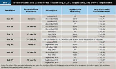
With the next three bear markets, Nov. 68, Jan. 73, and Nov. 80, all three portfolios returned to at least $100 in the exact same month. All three portfolios recovered from the Nov. 68 bear market in December of 1970, and all three were whole from the Jan. 73 bear market in June of 1975. In both cases, the 60/40 portfolio was worth slightly more than the 50/50 portfolios, which was worth slightly more than the NR portfolio.
The Nov. 80 bear market was curious because at the time that stocks had dipped 20 percent in July 1982, the portfolio was still valued at $103.04. In fact, as late as the rebalancing trigger point of November 1981, the original $100 was still worth $103.77. This was made possible by very high returns from bonds as rates came down from historic highs.
The one-day crash in October 1987 highlights the Aug. 87 bear market. Stocks did not recover as fast as they fell, but they recovered enough to result in more than a one-month differential in recovery times. The NR portfolio cracked $100 in January 1989 when it finished at $102.87, while the 50/50 portfolio made it in October 1988, and the 60/40 portfolio in September 1988. By the time the NR portfolio had recovered to $100, 50/50 was at $104.96, and 60/40 was at $107.21
The “lost decade” brought two severe bear markets and an end to the pattern observed in the first five bear markets where recovery dates and values were modestly better (at best) from rebalancing.
The tech wreck of March 2000 (the Mar. 00 bear market) was the only one of the seven bear markets that took longer than three years for the NR portfolio to return to a $100 value. Both the NR and 50/50 portfolios recovered in May 2003. The 60/40 portfolio, on the other hand, had recovered in November of 2001. However, 60/40’s value as of May 2003 was just $98.46; 50/50’s value was $100.46; and NR had the highest value at $103.02.
This was not what was observed with the Jan. 73 bear market. The difference is attributable to a slower and more modest increase in stock value over 2002 than the rapid rise in stock prices experienced during early 1975.
The Great Recession dominated the Oct. 07 bear market, and a similar value pattern resulted. The NR portfolio recovered to $102.52. At that same time, 50/50 was worth $101.51, and 60/40 just $100.39. Interestingly, all three first reached $100 again in September 2010.
Double Buys and Delayed Rebalancing
Some bear markets are more severe than others, dropping far below 20 percent. Therefore, consideration was given to two other rebalancing approaches.
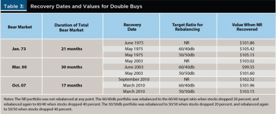
The first was to rebalance a second time (“double buy”) after stocks declined a cumulative 40 percent from the start of the bear market. So, when stocks dropped 20 percent, the portfolio was rebalanced to 50/50, and in the three severe bear markets of Jan. 73, Mar. 00, and Oct. 07, after stocks had slipped further to a cumulative 40 percent from their start, a second rebalance to 50/50 was made. The double buy for 60/40 would be done twice at the same trigger points also to 60/40. These are referred to in this analysis as 50/50db and 60/40db (see Table 3).
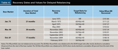
The second approach was to not rebalance at the down 20 percent trigger, but instead only rebalance after stocks had declined a cumulative 40 percent from the start of the bear market, called 50/50@-40 and 60/40@-40 in this analysis.
The Jan. 73 double buy for both the 50/50 target and the 60/40 target recovered only one month earlier than 50/50 and NR, but on NR’s recovery date, 60/40db was over $105, versus NR’s $101.86.
For Mar. 00, the double-buy method did not improve recovery time, and 60/40db even delayed recovery by a month.
For Oct. 07, both 60/40db and 50/50db recovered six months faster than 60/40, 50/50, and NR; and values exceeded 60/40 and 50/50 respectively, but 60/40db’s value actually lagged NR’s at the time NR recovered.
Delaying rebalancing until a bear market proved to be severe paid off in all three of the severe markets—Jan. 73, Mar. 00, and Oct. 07—with accelerated recoveries. For the Jan. 73 bear market, 50/50@-40’s recovery time was by a single month, and 60/40@-40’s was three months. In the other two severe bear markets, the recovery time was at least seven months faster.
Values for all rebalanced portfolios in all three severe bear markets were between $2.89 and $9.36 higher than NR’s values at the time the NR portfolio recovered (see Table 4).
Waiting for a bear market to become severe—down 40 percent in this case—appears to improve outcomes. However, it is reasonable to wonder if inaction over the many months it took each of the three severe bear markets to manifest would be overly stressful on clients.
To address this, a third strategy was considered. After a 20 percent decline, the portfolio was rebalanced back to its original 50/50 target. When the decline reached a cumulative 40 percent, the portfolio was then rebalanced to the more aggressive 60/40. This scenario is labeled “DA” for delayed aggression in the results shown in Table 6.
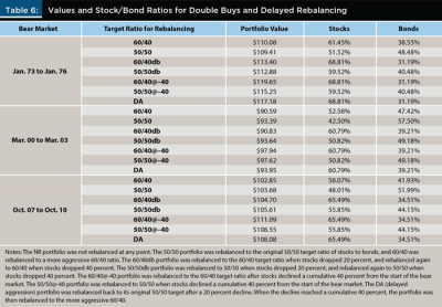
The results were mixed with recovery times and NR values not dramatically different. For the Jan. 73 events, this delayed aggression approach recovered in April 1975—two months faster than the NR portfolio—and was worth $108.93. The Mar. 2000 bear market was recovered by this strategy in the same month as NR with a similar value of $102.97. Only the Oct. 2007 scenario showed superior results, recovering six months faster than the NR portfolio and providing a value of $105.25 when NR returned to $100.
Values Three Years Out
For another angle on the effects of these methods, the analysis identified the values of the different scenarios three years from the commencement of the bear markets. For the first five bear markets, values three years from the start date were consistently higher for the 50/50 portfolio than the NR portfolio, and the 60/40 portfolio values were consistently higher than the respective 50/50 portfolio (see Table 5).
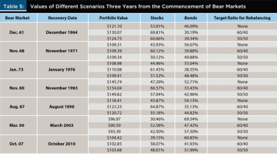
The two lost decade bear markets inverted the pattern with the NR portfolio holding higher values than the 50/50, which bested the 60/40.
Values three years out for the double buy strategies were better than the corresponding single buy scenarios, albeit barely when it came to the Mar. 00 bear market. The @-40 strategies resulted in significantly superior values for the Jan. 73 and Oct. 07 bear markets; and modestly for the Mar. 00 bear market. The delayed aggression approach also finished with generally better values than the NR, single buy, and double buy scenarios, but not as high as waiting to rebalance for the first time at –40 percent.
It is important to note that some of the stock/bond ratios at the end of three years approached 70/30. Whether a client with a 50/50 standard target would be comfortable enough with the higher allocations long enough to realize these benefits is debatable.
Further Research
Rebalancing to a more aggressive target allocation will likely appeal to some clients who feel emboldened by the mere act of rebalancing. However, these types of clients are likely to be in the minority. A larger population of clients is likely to reject the idea and either wish to stick to the original targets or not rebalance at all, especially in the face of a severe bear market. Nonetheless, additional questions for further research do arise:
- What are the effects of rebalancing to a more aggressive allocation for more conservative and more aggressive starting allocations such as 20/80 or 80/20?
- How do these rebalancing strategies fare with different trigger points?
- What would be the effects of shifting even more aggressively; i.e., from 50/50 to 70/30 instead of 60/40?
- How do these rebalancing strategies fare when multi-asset portfolios are used?
- Given the generally strong returns from bonds in many of these bear market situations, how would these rebalancing strategies fare when bond returns would likely be lower?
- How do these rebalancing strategies fare when modeled stochastically?
This analysis showed the effects of shifting allocation targets based on a 50/50 allocation at the commencement of a bear market. It is highly unlikely clients would have exactly a 50/50 mix at these points in time. Therefore, additional questions to explore in future research include: How do these rebalancing strategies fare when start dates are selected on a rolling basis? And, how would implementing these rebalancing strategies impact safe withdrawal rates?
Conclusions
This study provides general support to the conventional wisdom that during a bear market, holding is okay, and rebalancing is probably better. However, buying more equities than the amount indicated by the original target does not seem to substantially improve outcomes when the buying occurs upon a 20 percent decline. Some improvements in results were noted during severe bear markets when a second rebalance was performed. Additional improvement was observed when rebalancing to a more aggressive allocation was the only rebalancing performed deep into a severe bear market.
Only a modest acceleration of recovery times was observed at a rebalancing trigger point corresponding with the point a stock market decline first reached the traditional bear market status of down 20 percent.
During severe bear markets (–40 percent), the double buy method did not produce any improvement in recovery times, but it did yield some improvement in values three years after the beginning of the bear markets. The @-40 method materially improved recovery times, values at the time a never-rebalanced portfolio recovered, and values three years after the start of a bear market.
Implications for Financial Planners
Some clients do not have much flexibility with respect to the asset allocation that could serve them well. However, many clients who would choose a 50/50 allocation of stocks to bonds may find a 60/40 or 40/60 allocation to be reasonable, as well. For clients with some flexibility and a reasonable temperament or a desire for more proactivity, a more aggressive rebalancing approach may have appeal.
However, regardless of the rebalancing approach, if rebalancing does not occur close to the low point for equities during the bear market, clients will experience lower portfolio balances than if had they not rebalanced at all. During the Great Recession, a never-rebalanced portfolio dropped to $82.32 but rebalancing to 50/50 after a 20 percent decline in stocks resulted in a low value of $78.90. Rebalancing to a more aggressive 60/40 at that same time saw the value bottom out at $75.06.
In addition, more conservative or frightened clients are unlikely to be able to make the large shift to stocks required with a more aggressive rebalancing strategy, particularly in the face of a severe bear market and the resulting media attention that typically comes with market declines.
The most impactful rebalancing strategy observed in this analysis (60/40@-40), rebalanced only after the market declined 40 percent and then executed a move to a 60/40 target. This occurred at the end of November 2008. Before rebalancing, the portfolio held $29.66 of stock and $58.31 of bonds. So, to execute the most aggressive strategy and rebalance to 60/40, ($52.78/$35.19), $23.12, or 40 percent of the bond position, would need to be sold to buy stocks. That $23.12 buy represents a 78 percent increase to the stock holdings at the point of rebalancing.
It is not likely many clients would be able to take this approach. Most would find it difficult to wait for the –40 percent trigger point. Fewer still would then be able to execute such a dramatic shift.
As with other examinations of rebalancing, there are periods in which rebalancing enhances returns, but this study gives more credence to the idea that the primary purpose of rebalancing should be to maintain chosen exposures to various market risks.
A subtle implication is that the bond returns have a significant influence on account balances. If there had been losses in the bond portion of the portfolios, rebalancing would have lost its effectiveness in most cases. This implies that financial planners should be hesitant to chase yields by using long-term debt or holdings of weaker credits due to the potential volatility.
This study also supports the purported behavioral benefits of “doing something” during bear markets in that rebalancing during a bear market is not likely to result in an inferior outcome to not rebalancing at all. However, the improvements were generally so modest, it seems unlikely manipulating portfolio structure through aggressive rebalancing will be as impactful on goal achievement as other actions financial planners recommend to clients—such as saving more, spending less, managing taxation, or working longer.
Endnotes
- See the Investopedia article, “Warren Buffett: Be Fearful When Others Are Greedy,” at investopedia.com/articles/investing/012116/warren-buffett-be-fearful-when-others-are-greedy.asp.
- The seven bear markets were: (1) December 1961 to June 1962; (2) November 1968 to May 1970; (3) January 1973 to October 1974; (4) November 1980 to August 1982; (5) August 1987 to December 1987; (6) March 2000 to October 2002; and (7) October 2007 to March 2009. Source: “11 Historic Bear Markets,” from NBC News. Available at www.nbcnews.com/id/37740147/ns/business-stocks_and_economy/t/historic-bear-markets/#.XRT-W4hKjIV.
References
Bengen, William P. 1994. “Determining Withdrawal Rates Using Historical Data.” Journal of Financial Planning 7 (4): 171–180.
Bengen, William P. 1996. “Asset Allocation for a Lifetime.” Journal of Financial Planning 9 (8): 58–67.
Blanchett, David M. 2007. “Dynamic Allocation Strategies for Distribution Portfolios: Determining the Optimal Distribution Glide Path.” Journal of Financial Planning 20 (12): 68–81.
Blanchett, David M., Michael S. Finke, and Wade D. Pfau. 2014. “Asset Valuations and Safe Portfolio Withdrawal Rates.” Retirement Management Journal 4 (1): 21–34.
Campbell, John Y., and Robert J. Shiller. 1998. “Valuation Ratios and the Long-Run Stock Market Outlook.” Journal of Portfolio Management 24 (2): 11–26.
Daryanani, Gobind. 2008. “Opportunistic Rebalancing: A New Paradigm for Wealth Managers.” Journal of Financial Planning 21 (1): 48-61.
Davis, Joseph, Roger Aliga-Diaz, and Charles Thomas. 2012. “Forecasting Stock Returns: What Signals Matter and What Do They Say Now?” Vanguard Research. Available at www.vanguardcanada.ca/documents/forecasting-stock-returns.pdf.
Kitces, Michael E. 2008. “Resolving the Paradox: Is the Safe Withdrawal Rate Sometimes Too Safe?” The Kitces Report. Available at kitces.com/may-2008-issue-of-the-kitces-report.
Kitces, Michael E. 2009. “Dynamic Asset Allocation and Safe Withdrawal Rates.” The Kitces Report. kitces.com/april-2009-issue-ofthe-kitces-report-dynamic-asset-allocation-andsafe-withdrawal-rates.
Lee, Marlena 2008. “Rebalancing and Returns.” Dimensional Fund Advisors research. Available at citeseerx.ist.psu.edu/viewdoc/download?doi=10.1.1.625.3253&rep=rep1&type=pdf.
Pfau, Wade D. 2011a. “Can We Predict the Sustainable Withdrawal Rate for New Retirees?” Journal of Financial Planning 24 (8): 40–47.
Pfau, Wade D. 2011b. “Safe Savings Rates: A New Approach to Retirement Planning over the Life Cycle.” Journal of Financial Planning 24 (5): 42–50.
Pfau, Wade D. 2012a. “Long-Term Investors and Valuation-Based Asset Allocation.” Applied Financial Economics 22 (16): 1,343–1,353.
Pfau, Wade D. 2012b. “Withdrawal Rates, Savings Rates, and Valuation-Based Asset Allocation.” Journal of Financial Planning 25 (4): 34–40.
Pfau, Wade D., and Michael E. Kitces. 2014. “Reducing Retirement Risk with a Rising Equity Glide Path.” Journal of Financial Planning 27 (1): 38–45.
Citation
Moisand, Dan, and Mike Salmon. 2020. “Analyzing the Effects of Aggressive Rebalancing During Bear Markets.” Journal of Financial Planning 33 (1): 46–54.