Journal of Financial Planning: January 2013
Executive Summary
- Immediate fixed annuities (IFAs) are one of the oldest and most well-known products that can be used as a hedge against longevity risk for a retiree. Surveys show consumers like the fundamental attributes of annuities, yet a majority dislike annuities.
- This paper explores the potential benefits and true “cost” of IFAs based on various annuitization ages and scenarios. It uses two frameworks to achieve this: the internal rate of return (IRR) calculation, weighted for mortality, and a utility function.
- The paper first discusses the potential value of IFAs in terms of defined-contribution and defined-benefit plans. It shows that while longer life expectancies affect annuity payments, their overall impact is much less than the high correlation between bond yields and IFA rates.
- Using initial nominal withdrawal rates, the paper examines failure rates for straight life and period-certain IFAs for males, females, and joint couples. It finds that IRRs are similar across scenarios, but level off the longer the distribution period.
- The utility function (satisfaction) applied is the percentage of the total income goal replaced during retirement. Being able to replace only a smaller percentage of the need becomes increasingly costly at lower replacement levels.
- Given today’s low annuitization rates, many retirees are likely better off waiting until interest rates improve, or delaying the IFA purchase decision to an older age. IFAs also appear more attractive for individuals than couples. Nonetheless, IFAs remain an attractive longevity hedge for retirees age 80 or older, as well as for retirees who have a strong preference for guaranteed income and want to simplify the income-generation process, versus attempting to self-fund from a traditional retirement portfolio.
David M. Blanchett, CFP®, CLU, AIFA®, QPA, CFA, is the head of retirement research for Morningstar Investment Management in Chicago, Illinois. He has published more than 30 papers in various industry journals. (david.blanchett@morningstar.com).
Longevity risk, or the risk of outliving one’s assets, is a concern of many retirees. Financial advisers employ a variety of tools to hedge against longevity risk. One of the most common is to purchase an annuity that guarantees lifetime income. The simplest annuity form is an immediate fixed annuity (IFA) where the annuitant “trades” a lump sum of cash for a stream of lifetime income guaranteed by the annuity company.
Because annuities are a form of insurance provided by for-profit companies, the “average” annuitant should not expect to come out ahead when buying an annuity. However, it may still be possible for the annuitant to experience a positive expected value based on that person’s subjective life expectancy, interest rate assumptions, or from a utility perspective. This paper will explore the potential benefit of immediate fixed annuities for males, females, and joint couples based on various annuitization ages and scenarios to help advisers and their clients understand the true “cost” of these annuities and when they work best for a retiree.
Why Annuities Can Make Sense
One way to explain to clients the potential value of IFAs is to discuss them in terms of defined-contribution and defined-benefit plans. Defined-contribution plans are less effective than defined-benefit plans when viewed from the perspective of a maximization of a participant’s lifetime income, because defined-benefit plans pool longevity risk while defined-contribution plans force employees/participants to individually deal with longevity risk.
For example, take a retirement plan with 100 employees, all males age 65. Total plan assets are $100 million and each employee’s fractional share is equal (that is, each has a “balance” of $1 million). All payments/distributions are set to commence one month from today, and the expected return on assets is 5 percent. The life expectancy for a 65-year-old male is 17 years (age 82) according to the 2007 Social Security Administration table. If we assume the retirement plan is a defined-benefit plan, longevity risk can be pooled across participants and benefits determined accordingly. Using a conservative distribution of 20 years (life expectancy + three years) each participant in the defined-benefit plan would be expected to receive a monthly income benefit of $6,690 based on a simple time-value-of-money calculation.
In contrast, with a defined-contribution plan, such as a 401(k), each participant will have to “self-fund” his or her retirement income. If we assume each participant plans to draw income from the portfolio (versus buying a guaranteed lifetime income), it is unlikely each participant will use a 20-year (age 85) retirement period estimate because the probability of a 65-year-old male living past age 85 is 40 percent. If we use a more conservative death age, such as age 90, which has a 20 percent probability of outliving the distribution period, the expected monthly income would decrease from $6,690 to approximately $5,915. Moreover, that lower amount includes a 20 percent chance each participant in the 401(k) plan will run out of money at age 90, while the income from the defined-benefit plan is guaranteed for life.
The trade-off between the approaches is that should the participant in a defined-contribution plan die shortly after retiring, the portfolio balance can be passed along to his or her heirs. No such balance exists in a defined-benefit plan, however, because the benefit is based in the form of lifetime income (or joint life if it’s in the form of survivor benefits). Therefore, defined-contribution participants (or really non-annuitizers) are trading the potential benefit of guaranteed lifetime income for the possibility of dying early in retirement.
The “cost” associated with dying early during the annuitization period can be offset by adding riders, such as return of premium or period-certain payments. These riders contain additional embedded costs, however, which need to be considered before selecting them.
Why Not Annuities?
If the objective is to maximize guaranteed lifetime income, the defined-benefit plan is clearly the optimal choice. Unfortunately, as advisers well know, defined-benefit plans are dying off in America (at least among large employers) because employers don’t want the additional risk associated with funding defined-benefit plans. This has led to a massive shift to 401(k) and other types of defined-contribution plans. Annuities are one obvious way to solve the longevity-risk puzzle within a defined-contribution plan. The public, however, (and for that matter, many financial planners) historically has not had a favorable view of annuities.
For example, a survey conducted by Allianz Life Insurance Company of North America (Bhojwani) noted that nearly 54 percent of Americans age 44–75 expressed distaste for the word “annuity.” Consumers find annuities complex, along with egregious surrender penalties, transfer restrictions, and sales by commissioned agents who are not required to serve as fiduciaries. Yet interestingly, 80 percent of those surveyed preferred a product with 4 percent return and a guarantee against losing value over a product with 8 percent return but subject to market risk. Clearly, those surveyed like the fundamental attributes of an annuity. It’s the practical implementation that has caused such problems.
Annuities Today
When annuitizing, the actual income benefit received by the annuitant is based on two primary factors: life expectancy and interest rates. Life expectancy sets the basis for how long the annuitant (or annuitants) is expected to live. The longer someone is expected to live, the lower the annuity payment. Interest rates indicate the approximate returns the insurance company can earn on its investments; lower interest rates mean lower annuity payments because the insurance company earns less on its capital.
Even though life expectancies continue to increase, their overall effect in recent history has been less pronounced on benefit payments than interest rates. Figure 1 includes information about historical immediate annuity rates as a percentage of the purchase price for a 65-year-old male and female versus the yield on the Barclays U.S. Treasury 20+ Year Index over the last 25 years. (Note, while immediate annuity income is usually expressed in the form of a monthly benefit in dollar terms, this paper uses annual income as a percentage of purchase price approach to make the benefit more comparable to initial sustainable withdrawal rates from a distribution portfolio, such as 4 percent).
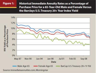
Figure 1 demonstrates the strong relationship between bond yields and immediate annuity rates, with a correlation of 0.94 during the period. Interest rates and bond yields have trended lower versus long-term averages, and annuity yields have followed suit.
Table 1 shows data about current IFA rates, which are the best possible annuitization rates available, obtained through immediatennuities.com in February 2012. Table 1 shows the monthly income for a $100,000 initial premium, as well as the annual income as a percentage of the purchase price for a male, female, and joint couple (both the same age, with a 100 percent survivor benefit) for various annuitization ages. Two types of annuity rates are used: one is for a straight life annuity, which pays a benefit for the life of the annuitant or both lives of joint annuitants, and the second rate is for a life annuity with a 10-year certain payment, where the annuitant receives a reduced lifetime benefit (versus the life-only annuity) but is guaranteed to receive at least 10 years of payment (either by the annuitant or the annuitant’s beneficiary).
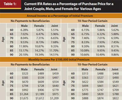
Immediate fixed annuity rates are higher for older annuitants and higher for males than females because of shorter life expectancies. A joint couple annuity has the lowest payout because both annuitants must die before the annuity stops paying a benefit. Straight life annuities without a period-certain guarantee provide more income because the participant risks dying shortly after annuitization, receiving little or no benefit.
The “cost” of the 10-year certain payment also increases for older annuitants. For example, a 60-year-old male can receive $523 a month from a life annuity, while the monthly income from a life annuity with a 10-year period certain drops only $10 to $513 a month. Contrast that to the annuity payout rates for a 90-year-old male, where the 10-year period certain annuity produces an income level about half of the life annuity.
Sustainable Withdrawal Rates
Past research on sustainable withdrawal rates primarily has been based on maintaining a constant inflation-adjusted withdrawal amount during retirement. For example, if the initial portfolio value is $1 million, an initial withdrawal rate of 4 percent would generate $40,000 in income the first year. That initial withdrawal amount is then adjusted each year for inflation. If inflation is 3 percent in the second year, the withdrawal amount would be assumed to increase to $41,200.
The income from immediate annuity benefits is not usually adjusted for inflation. A recent LIMRA study noted that 93 percent of income annuity contracts have no automatic payment increase (or cost-of-living adjustment rider). Therefore, initial nominal withdrawal rates provide a better reference point when establishing a probability of failure than initial real withdrawal rates. The probability of failure for a real withdrawal scenario (for example, 4 percent of the initial balance) is going to be higher than a nominal withdrawal scenario because the cash flows from the real withdrawal scenario increase through retirement (by inflation) while the cash flows from the nominal scenario are constant. The differences in probabilities of failure for nominal versus real initial withdrawal rates for various periods are included in Table 2. The probabilities of failure are based on 10,000 Monte Carlo simulations for a portfolio that has a lognormal distribution with a mean return of 7 percent and a standard deviation of 9 percent (approximately a 40 percent equity portfolio). A more conservative portfolio is used for the analysis to better reflect the actual equity allocations of retirees, who tend to allocate approximately 25 percent of their financial assets to equities, on average, based on the 2010 Survey of Consumer Finances data. Inflation is assumed to be 3 percent for the real withdrawal scenarios.
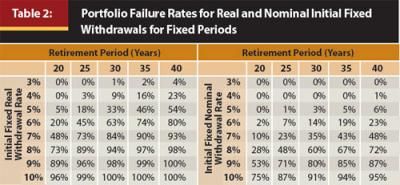
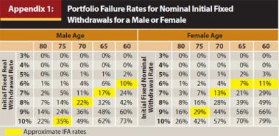
While the failure rate of the 30-year, 4 percent initial real withdrawal scenario is 9 percent, the failure rate of the nominal withdrawal scenario is zero. Not surprisingly, the nominal withdrawal scenarios have failure rates that are considerably smaller than the real withdrawal scenarios. Calculating the probability of failure over some fixed period, though, such as 30 years, ignores what actually constitutes “failure” from a lifetime income perspective, which is a portfolio no longer able to support lifetime income and the retiree is still alive. This is a concept that has been discussed previously by Blanchett and Blanchett (2008). Appendix 1 includes the probabilities of the portfolio not being able to sustain an initial withdrawal rate while either a male or female retiree is still living.
Portfolio Failure Incorporating Life Expectancy
When portfolio failure is viewed from the perspective of the retiree still being alive and the portfolio no longer able to sustain the withdrawal amount, failure rates decrease considerably, as both actions must occur for the portfolio to be considered a failure. Table 3 includes information about the probabilities of failure for a joint couple, male and female both the same age, where life expectancy data is based on the Annuity 2000 Mortality Life Table (for more details on the Annuity 2000 tables, see Appendix 2). The probability of dying each year is calculated independently for the male and female. The portfolio is considered to have “failed” only if the portfolio value cannot sustain the withdrawal rate and either member of the couple is still living. Each scenario is based on a 10,000-run Monte Carlo simulation using the same return assumptions for the calculations for Table 2.
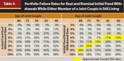
Table 2 can be directly compared with Table 3 based on using age 100 as the target “death age” for a couple. Under this concept, the length of the retirement period is determined by subtracting the joint age of the couple from 100. Using age 100 as the target was a subjective decision by the author, based on the fact the probability of outliving the target age was approximately 15 percent for each of the different age combinations. For example, a couple both 65 years old would use a 35-year distribution period because 100 minus 65 is 35.
Incorporating life expectancy into the definition of failure has a considerable impact on portfolio failure rates. In every scenario, the probability of portfolio failure decreases when considering joint life expectancy. For example, the 35-year, 6 percent initial real withdrawal scenario (in Table 2) has a 74 percent probability of failure. In contrast, the probability of a couple both age 70 running out of money while either member of the couple is still living, assuming a 6 percent initial real withdrawal (Table 3), is only 50 percent. The probability of failure for life expectancy nominal withdrawal of 6 percent is only 11 percent.
These results are important, especially the nominal rates, because it better frames the respective potential benefit of an annuity versus self-funding retirement income. For example, the percentage income of the initial premium for an annuity bought by a joint couple, both age 65, with a 100 percent survivor benefit, is 5.88 percent. This approximately corresponds to an 11 percent probability of failure for the “nominal withdrawal” table in Table 3. Note, though, that the corresponding probability of failure increases at older ages. This relationship is also evident in Appendix 1, which includes the corresponding probabilities of failure during the lifetime for a male or female for a nominal withdrawal rate. Therefore, the relative attractiveness of an IFA is not constant through time. This is something that must be considered when determining the appropriate time to annuitize.
Assessing the True Cost of an Annuity
It’s important that a potential purchaser understand that an annuity is a form of insurance that should not be expected to have a positive average expected value, and will therefore compare unfavorably to non-annuity portfolios in “average” scenarios. The annuity “pays off” only if the annuitant lives longer than he or she is expected to live. Therefore, the potential cost of an IFA (or really any form of guaranteed income product) should be expressed in a way that helps the potential purchaser understand whether the potential benefit is worth the cost.
For example, if the value of your home is $100,000 and the probability of it burning down is 1 percent (per year), the insurance portion of fire insurance for your home would be $1,000. Given that insurance companies have additional expenses and are supposed to turn a profit, we would expect the premium to be more than $1,000. The additional cost affects the attractiveness of the insurance. If the insurance costs $1,200, it’s probably a good deal; if it costs $2,500, some people may be less inclined to buy the insurance, especially if those individuals have a large amount of savings and can afford the loss (at least to some extent).
The payments received by an annuitant from an IFA can be broken down in three parts: interest, return of premium, and mortality credits. The relationship of these adjusts throughout retirement. The interest and return of premium are the components a retiree could earn if he or she decided to “self-fund” retirement income. The mortality credit is the “benefit” received by an annuitant that is subsidized by the mortality experience of the mortality pool, since those who die early subsidize those who live a long time. This is also known as the “mortality premium.”
In perhaps one of the first pieces to directly discuss the potential benefits of immediate annuities, Yaari (1965) noted that under some specific assumptions rational individuals with no bequest motive should convert all of their retirement wealth to an annuity at retirement. Yaari shows that by buying an annuity you assure yourself a higher level of consumption in every year that you live, compared with holding a bond with a similar risk profile. The goal of the remainder of this paper is to help the reader better understand the potential benefits associated with an IFA from both an individual investment perspective, as well as within the framework of a total portfolio.
Analyzing the Benefit
The longer the annuitant receives annuity payments, the higher the return on investment the annuitant is going to realize. This is common sense to a certain extent, as the total number of annuity payments received by the annuitant is the effective “gamble” the annuitant is taking when buying the annuity. The actual return achieved by the annuitant can be measured by calculating the internal rate of return (IRR). The IRR is the discount rate that makes the net present value of the cash flows from a particular investment equal to zero, or more simply, is the actual rate of return realized by the investor on the investment. Figure 2 includes the IRRs for male, female, and joint couple (both the same age, 100 percent survivor benefit) for various annuity payment years based on current IFA rates (Table 1) assuming annuitization at age 65. The figure shows the IRRs for a straight life annuity and 10-year period certain.
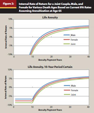
The first thing the reader should note about Figure 2 is that the internal rates of return are very similar across the scenarios for the male, female, and joint scenarios for both types of annuities. Given current IFA rates, the IRR for each of the three scenarios, male, female, and joint couple, are all positive by approximately age 80, or 15 years into annuitization. Something to note, though, is that IRRs increase at a decreasing rate. The IRRs increase rapidly initially and then level off the longer the distribution period.
The income derived from a male IFA is higher than a female IFA or joint IFA, because of a shorter life expectancy. For example, the probability of a 65-year-old male living to age 82 is approximately 64 percent, while the probability for a 65-year-old female is approximately 75 percent, or 11 percent higher. A male annuitant also bears the most risk when it comes to IFA annuitization payoff. There is a 0.6 percent chance a 65-year-old male will not live to age 66 (die within a year). Under this scenario, if the annuity cost $100,000 the income received would only be $6,280, which is a rate of return of −93 percent.
Alternatively, assuming life expectancies are independent, there is only a 0.006 percent chance that at least one member of a joint couple, both age 65, will not live to age 66. This makes annuitization a much less risky proposition for a couple, from the perspective of dying early in the annuitization and effectively achieving a very negative IRR. The distribution of IRRs for a Monte Carlo simulation for a 65-year-old joint couple, female, and male IFA, based on current rates (in Table 1) are included in Figure 3 to give the reader a better idea of the expected “payoff” of annuitization.
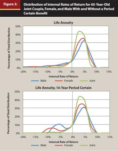
The IRR distributions in Figure 3 are clearly not normal, which means they do not take the shape of a bell curve. The distributions for the life annuity exhibits a high level of negative skewness, which can be attributed to the return implications of dying early during the IFA period. While the probability of dying a few years into annuitization may be low, if it occurs it results in a significant loss to the annuitant (from an investment perspective). This is why most annuities sold include some type of return of premium feature, such as a term certain rider that ensures at least some minimum portion of the original purchase price is refunded. This creates a minimum rate of return that can be expected to be earned by the annuitant. For example, the minimum IRR for the life annuity with a 10-year period certain male scenario in Figure 3 is −6.6 percent. The guarantee of 10 years of payments creates a bimodal distribution, because every annuitant (or beneficiary) who dies within the first 10 years would receive the same cash flows regardless of how long the annuitant and beneficiary live.
From a practical perspective, the negative skew associated with IRRs in Figure 3 should be viewed as the “cost” of offsetting the potential positive skew associated with life expectancy. The annuitant is effectively trading the possibility of dying early (and the corresponding negative IRRs) with the hedge of living a long life and having guaranteed income the entire period.
Because the shape of the IRR distribution for immediate annuities in Figure 3 is non-normal, there are considerable differences in the average return and median returns for various IFAs. Not surprisingly, the median return is always higher than the average return because the median isn’t influenced by outliers. For example, while the median return for a 65-year-old male based on current rates is 3.8 percent, the average is −1.0 percent. The difference in the values (4.8 percent) is because of the possibility of the male dying very early in the distribution period, not realizing the full potential benefit of the annuity.
Utility Framework
Because it is difficult, if not impossible, to model the exact risk preferences of retirees, one approach is to introduce the notion of “utility,” where one can quantify the satisfaction achieved from some given event or action. The objective is to maximize the utility (satisfaction) based on the different options available. One common theory of risk preference, constant relative risk aversion (CRRA), is depicted in the following formula:
For a utility function to be valid, however, it must effectively convey the actual preferences of the individual it’s reflecting. For this analysis, the utility maximizing value (the “x” in the equation) is the percentage of the total income goal replaced during retirement. This is calculated by dividing the net present value of all payments received over the retiree’s lifetime plus the total balance of assets at death, by the net present value of the total income need. Based on this methodology, it is possible to have a replacement amount greater than 100 percent if there are assets remaining upon the death of both retirees.
Including the total assets at death incorporates the trade-off a retiree would potentially make by buying an IFA with retirement assets. The lack of a guarantee (income stability), therefore, must be worth the potential upside of having more assets at death to warrant not making the trade. While the motives for bequest versus maximizing lifetime income may differ, focusing on the income component of an IFA alone would overly penalize a strategy with a balance remaining at retirement. While one approach would be to use a subject-weight measure to gauge the investor’s preference for income versus bequest, the analysis assumes the investor has a high bequest preference, thus making the IFA less attractive.
The annual income need is assumed to be a constant real value, increasing by 3 percent a year for inflation. Therefore, the IFA will consist of a decreasing percentage of the retiree’s need as the retirement period progresses. The discount rate for all net present value calculations is 5 percent, which is the assumed return on bonds. While it potentially would make sense to use a lower discount rate for income sources that are guaranteed (such as IFA and pension income) versus those that are not (say, portfolio income), a constant discount rate is used so as to not favor the IFA. The income need is assumed to exist as long as either member of a couple is still living.
For the equation, the risk-aversion level (gamma or Υ) is set at four, which indicates a moderate level of risk aversion. The key idea behind the utility approach is that being able to replace only a smaller percentage of the total need becomes increasingly costly at lower replacement levels. While it is certainly good to build a large surplus, the utility-maximizing portfolio will be the combination of assets that both maximizes retirement income and minimizes the downside variability associated with generating the income. This is a very similar to an approach taken by Chen and Milevsky (2003) when seeking to determine the optimal allocation to guaranteed products.
Allocating to an IFA Within a Total Portfolio Framework
The portfolio is assumed to have a nominal return of 7 percent and a standard deviation of 9 percent, which is the approximate long-term return of a 40-60 equity/bond portfolio. Returns are lognormally distributed. Inflation is assumed to be a constant 3 percent a year. Each scenario assumes the retiree has a balance of $500,000 in assets and an annual, inflation-adjusted pension benefit of $30,000 a year with a full survivor benefit. The pension benefit is assumed to have a perfectly offsetting liability (that is, the $500,000 is funding additional potential income), therefore, the pension benefit serves as a floor to the replacement percentage for the utility calculation, which is approximately 50 percent. The benefit is the same regardless of whether the scenario is male, female, or joint. The pension is assumed to last the entire distribution period; therefore, it has a 100 percent survivor benefit for the joint scenario.
IFA allocation ranges are tested between zero and 100 percent in 10 percent increments for each of the tests (11 scenarios). Male, female, and joint couple scenarios, for both a life-only annuity and a life-only annuity with a 10-year period certain (six scenarios), are tested for ages 60, 65, 70, 75, and 80 (five scenarios). Withdrawal rates from 3 percent to 8 percent in 1 percent increments are considered (six scenarios), for a total of 1,980 scenarios. Withdrawals are assumed to come from
the annuity first and then the portfolio.
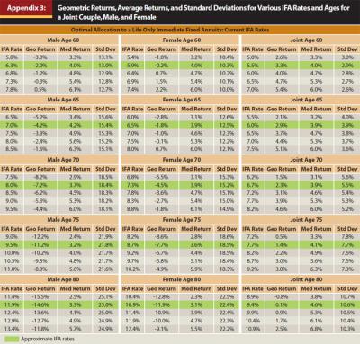
If the annuity can fund more than the required withdrawal, the excess is assumed to be saved in the portfolio. While an 8 percent initial withdrawal is an incredibly aggressive withdrawal rate for a 60-year-old joint couple, it is less so for an 80-year-old male. Results are also included for current IFA rates, as well as current rates +50 bps and +100 bps to reflect the potential change in relative attractiveness should IFA rates increase with interest rates. The results are included in Table 4. The median geometric returns, average returns, and standard deviations for the various IFA scenarios considered are included in Appendix 3.
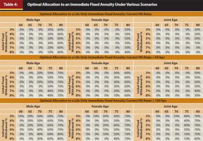
Based on the IFA allocations in Figure 3, IFAs do not appear that attractive on a relative basis within a total portfolio framework, especially for younger retirees1. An IFA is not featured for any of the current rate scenarios under age 70, and only with material allocations for those annuitizing at age 80. However, the optimal allocation to an IFA does increase at older ages, and increases considerably should IFA rates improve. The allocation to IFAs improved for older retirees regardless of the scenario. Note, IFAs appear to be more attractive for individuals (males and females) than joint couples on a relative basis. The results are obviously going to be sensitive to the assumptions, in particular the portfolio return/risk assumptions, the level of pension income, the level of risk aversion, and the IFA rates.
Conclusion
Immediate fixed annuities are one of the oldest and most well-known products that can be used as a hedge against longevity risk for a retiree. This paper uses two frameworks to help the reader better understand the potential benefits and costs of an IFA: the internal rate of return (IRR) calculation, weighted for mortality, and a utility function.
Given today’s annuitization rates, which are currently near all-time lows, many retirees are likely better off waiting until interest rates and subsequent annuitization rates improve, or delaying the IFA purchase decision to an older age. Even with today’s low rates, IFAs remain an attractive longevity hedge for retirees age 80 or older, as well as for retirees who have a strong preference for guaranteed income and want to simplify the retirement income generation process, versus attempting to self-fund from a traditional retirement portfolio.

Endnotes
- Milevsky and Chen (2003) noted significantly higher allocations to IFAs, yet this a function largely of the different rates available at the time of their writing, which were approximately 30 percent higher, or +150 bps, than the rates available at the time of this writing.
References
Bhojwani, Gary C. 2011. “Rethinking What’s Ahead in Retirement.” Allianz Life Insurance Company of North America.
Blanchett, David M., and Brian C. Blanchett. 2008. “Joint Life Expectancy and the Retirement Distribution Period.” Journal of Financial Planning 21, (December): 54–60.
Chen, Peng, and Moshe Milevsky. 2003. “Merging Asset Allocation and Longevity Insurance: An Optimal Perspective on Payout Annuities.” Journal of Financial Planning, 16, (June): 52–63.
Federal Reserve. 2010. “2010 Survey of Consumer Finances.” www.federalreserve.gov/econresdata/scf/scf_2010.htm
LIMRA. 2010. “Guaranteed Income Annuities Report.” www.limra.com/newscenter/newsarchive/archivedetails.aspx?prid=157
Yaari, Menahem. 1965. “Uncertain Lifetime, Life Insurance, and the Theory of the Consumer.” Review of Economic Studies 32, 2: 137–150.