Journal of Financial Planning: January 2012
Executive Summary
- Most retirement withdrawal rate studies are based either on historical data or use a particular assumption about portfolio returns unique to the study in question. But planners may have their own capital market expectations for future returns from stocks, bonds, and other assets they deem suitable for their clients’ portfolios. These uniquely personal expectations may or may not bear resemblance to those used for making retirement withdrawal rate guidelines.
- The objective here is to provide a general framework for thinking about how to estimate sustainable withdrawal rates and appropriate asset allocations for clients, based on one’s capital market expectations, as well as other inputs about the client including the planning horizon, tolerance for exhausting wealth, and personal concerns about holding riskier assets.
- The study also tests the sensitivity of various assumptions for the recommended withdrawal rates and asset allocations, and finds that these assumptions are very important.
- Another common feature of existing studies is to focus on an optimal asset allocation, which is expected either to minimize the probability of failure for a given withdrawal rate or to maximize the withdrawal rate for a given probability of failure. Retirement withdrawal rate studies are known in this regard for lending support to stock allocations in excess of 50 percent.
- This study shows that usually there is a wide range of asset allocations that can be expected to perform nearly as well as the optimal allocation, and that lower stock allocations are justifiable in many cases.
Wade D. Pfau, Ph.D., CFA, an associate professor at the National Graduate Institute for Policy Studies in Tokyo, Japan, holds a doctorate in economics from Princeton University. His hometown is Des Moines, Iowa. He can be reached at wpfau@grips.ac.jp.
Most retirement withdrawal rate studies are based either on the historical data parameters from Ibbotson Associates’ Stocks, Bonds, Bills, and Inflation (SBBI) data since 1926 or on some other variant of the historical data, or they use a particular assumption about market returns unique to the study. Guidelines from such studies may not fulfill the needs of planners who develop their own capital market expectations for a wide variety of asset classes they and their clients deem suitable. These personal expectations may or may not bear close resemblance to the expectations built into existing retirement withdrawal rate guidelines. Not only might planners hold views about future stock and bond returns that are different from historical averages but also planners may include other assets such as TIPS, international stocks and bonds, REITs, and commodities, for instance. Lack of sufficient data often prevents the inclusion of such asset classes in withdrawal rate studies.
Another common feature of existing studies is to focus on an optimal asset allocation, which is expected either to minimize the probability of failure for a given withdrawal rate or to maximize the withdrawal rate for a given probability of failure. Studies have tended to support stock allocations for retirees in excess of 50 percent. The framework for this study shows that usually there is a wide range of asset allocations that can be expected to perform nearly as well as the optimal allocation, and that lower stock allocations are justifiable in many circumstances.
The objective of this study is to provide a framework for thinking about how to estimate sustainable withdrawal rates and appropriate asset allocations for clients based on a planner’s capital market expectations and asset choices, as well as other inputs about the client including the planning horizon, tolerance for exhausting wealth, and personal concerns about holding riskier assets. The study also includes an investigation of the sensitivity of various assumptions and their effects on the results. The study concludes by combining these elements with a hypothetical example to translate capital market expectations into recommendations for a sustainable withdrawal rate and asset allocation strategy. With this framework, planners no longer remain captive to the capital market expectations used in various withdrawal rate studies and will have a method for including any desired asset classes.
Literature Review
We can classify existing withdrawal rate studies into several categories. First are studies investigating the issue with overlapping periods from the historical data. The most common historical data are Ibbotson Associates’ Stocks, Bonds, Bills, and Inflation (SBBI) data for total returns in U.S. financial markets since 1926. Studies of this nature tend to support a relatively high stock allocation in retirement and tend to provide the strongest support for the safety of the 4 percent rule. For instance, the seminal Bengen (1994) article concludes that retirees in all historical circumstances could safely withdraw 4 percent of their assets at retirement and adjust this amount for inflation in subsequent years for a 30-year retirement duration. Using the S&P 500 and intermediate-term government bonds, he determines that retirees are best served with a stock allocation between 50 and 75 percent, concluding that “stock allocations below 50 percent and above 75 percent are counterproductive.” Several years later, Cooley, Hubbard, and Walz (1998) augment Bengen’s work to show success rates for different withdrawal rates and asset allocations also using overlapping historical simulations. Recently, Cooley, Hubbard, and Walz (2011) updated their earlier findings, also concluding that retirees are best served with stock allocations of at least 50 percent. From their tables, a 75 percent stock allocation maximizes the success rates for 30 years of inflation-adjusted withdrawals using a 4 percent or 5 percent withdrawal rate. Bengen (1996) had already noted, however, that with rolling 30-year periods from the historical data, withdrawal rates above 4 percent could have been supported with asset allocations ranging between 35 percent and 90 percent stocks. In other words, retirees fearing high stock allocations could reduce their stock allocations below 50 percent with minimal impact on their sustainable withdrawal rates.
A second approach to studying withdrawal rates is to use Monte Carlo simulations, which are parameterized to the same historical data as used in historical simulations. This can be done either by randomly drawing past returns from the historical data to construct 30-year sequences of returns in a process known as bootstrapping, or by simulating returns from a distribution (usually a normal or lognormal distribution) that matches the historical parameters for asset returns, standard deviations, and correlations. This simulation approach has the advantage of allowing for a wider variety of scenarios than the rather limited historical data can provide (between 1926 and 2010, there are only 56 rolling 30-year periods). In this regard, Monte Carlo simulation studies of this nature generally show slightly higher failure rates for stock allocations in the 50 to 75 percent range. At the same time, if past returns are not reflective of the distributions for future returns, these Monte Carlo simulations will suffer from the same deficiency of misestimating the sustainability of various withdrawal rates.
Another advantage of Monte Carlo simulations, relative to historical simulations, though, is that because of the way overlapping periods are formed with historical simulations, the middle part of the historical record plays an overly important role in the analysis. With data since 1926, this overweighted portion (1955–1981) of the data tends to coincide with a severe bear market for bonds. Monte Carlo simulations treat each data point equally, and simulations based on the same underlying data tend to show greater success for bond strategies and lower optimal stock allocations than historical simulations. Probably the best demonstration of this particular Monte Carlo simulation approach is Spitzer, Strieter, and Singh (2007), who provide illustrations for how withdrawal rates, asset allocations, failure probabilities, and bequest motives all interact for a 30-year retirement duration with simulations based on the historical data. Williams and Finke (2011) also use bootstrapped simulations with the historical data since 1926 to investigate optimal withdrawal rates and asset allocations in a utility-maximizing framework.
A third category includes studies using Monte Carlo simulations based on different parameters than the historical data, either because the authors are incorporating their own expectations about future returns or because they seek to illustrate a basic concept with simple return assumptions. An excellent study of this nature that serves as a precursor of the present study is Blanchett and Blanchett (2008). They make the point that future returns for a 60/40 portfolio could be even one or two percentage points less than historical averages, and they show how portfolio failure rates relate to changes in both the assumed return and standard deviation. Saltzman (2006) also demonstrates how withdrawal rates are sensitive to portfolio returns and volatilities using several different assumptions for these values in a Monte Carlo framework. Milevsky and Abaimova (2006) also assess portfolio success rates assuming stocks earn a real arithmetic return of 7 percent with 20 percent volatility, and bonds earn 2.5 percent with 10 percent volatility.
More recently, Van Harlow (2011) analyzes asset allocation in retirement using a downside risk perspective that moves beyond failure rates to quantify the degree of failure as well. He determines that stock allocations between 5 percent and 25 percent work best. These low stock allocations result not only from the assumed conservative nature of the retiree but also from Van Harlow basing Monte Carlo simulations on lower real stock returns and higher real bond and bill returns than the historical averages.
Also relevant, Athavale and Goebel (2011) investigate retirement success over 35 years using 10 different assumptions for the underlying distribution of portfolio returns that average 5.1 percent in real terms with a 12 percent standard deviation. They only use 10 simulations for each distribution, but with the limited sample they find the lowest withdrawal rate is 2.52 percent, and that 4 percent withdrawals fail 14 percent of the time over a shorter 30-year period across the 100 simulated scenarios.
Finally, Huebscher (2011) provides an example of specifically simulating the potential success for an all-TIPS strategy over a 30-year period. Real TIPS yields start from their most recent value, and results are tested for several assumptions about their volatility.
Methodology
The maximum sustainable withdrawal rate (MWR) is the highest withdrawal rate that would have provided a sustained real income over a given retirement duration and for a given failure rate. At the beginning of the first year of retirement, an initial withdrawal is made equal to the specified withdrawal rate times the accumulated wealth. Remaining assets grow or shrink according to the asset returns for the year. At the end of the year, the remaining portfolio wealth is rebalanced to the targeted asset allocation. In subsequent years, the withdrawal amount adjusts by the previous year’s inflation rate and the order of portfolio transactions is repeated. Withdrawals are made at the start of each year, and the amounts are not affected by asset returns, so the current withdrawal rate (the withdrawal amount divided by remaining wealth) differs from the initial withdrawal rate in subsequent years. If the withdrawal pushes the account balance to zero, the withdrawal rate was too high, and the portfolio failed. The MWR is the highest rate that succeeds. Taxes are not specifically incorporated, and any taxes would need to be paid from the annual withdrawals.
Monte Carlo simulations are performed using a lognormal distribution for (1 + return). Ten thousand simulations are made for each of 2,156 combinations of underlying portfolio real returns and standard deviations. Average real arithmetic returns range in 0.25 percentage point increments from –2 percent to 10 percent, and standard deviations range in 0.5 percentage point increments from 0.5 percent to 22 percent. For retirement durations of 10 to 40 years in 5-year increments, the MWR is calculated for each of the 10,000 simulated return paths from each of the 2,156 return/volatility combinations. With these outcomes, failure rates can be estimated for a given withdrawal rate, or the maximum withdrawal rate can be identified for a given chance of failure. These simulated return-risk combinations provide a grid of outcomes, and I use linear interpolation between the nearest neighbors on the grid to estimate the MWR for portfolios with other returns and volatilities.
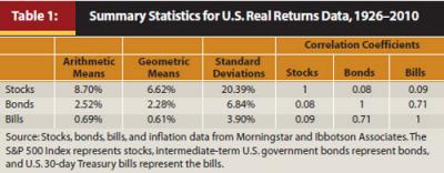
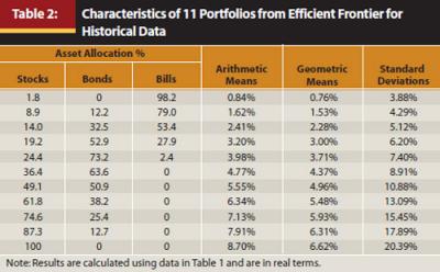
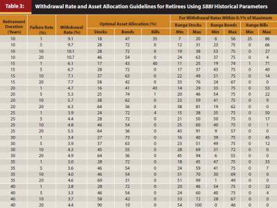
To consider how capital market expectations affect withdrawal rates and asset allocation, planners can identify the expected real arithmetic returns, standard deviations, and correlations between assets that they intend to include in their clients’ portfolios. For planners wishing to use historical data parameters, Table 1 provides this information for large-capitalization stocks, intermediate-term government bonds, and Treasury bills. With the chosen inputs, the next step is to generate 100 points on the efficient frontier using standard mean-variance optimization methods. This optimization identifies the asset allocations providing the highest returns for a given risk, or the lowest risk for a given return. I assume no leverage or short selling, so each asset is bound between 0 and 100 percent of the portfolio. Table 2 provides details for 11 arbitrary portfolios taken from the efficient frontier for the asset characteristics in Table 1. The efficient frontier can then be plotted onto the grid that relates returns and risks to withdrawal rates, and the asset allocation supporting the highest withdrawal rate can then be identified from the graph. In addition to the optimal asset allocation, I will identify asset allocations supporting withdrawal rates within 0.1 percentage points of the MWR as well.
Capital Market Expectations and Safe Withdrawal Rates
Figure 1 shows how the frequency of failures for a 4 percent withdrawal rate over a 30-year retirement horizon relate to the arithmetic average real returns and standard deviations provided by the underlying portfolio. Naturally, higher real returns and smaller volatilities contribute to smaller failure rates. For instance, if portfolio returns experience a standard deviation of 12, reducing the real return from just over 6 percent to just over 4 percent would increase the failure rate from 5 percent to 20 percent. Or, for instance, if the portfolio return averaged 4 percent, increasing the standard deviation from 7 percent to about 11.5 percent would also increase the failure rate from 5 percent to 20 percent. For smaller failure rates, returns must be increased at a faster pace to offset the impact of increasing standard deviations. Figure 1 also includes a red curve representing 100 points from the efficient frontier for a portfolio exhibiting the historical characteristics shown in Table 1. Though the asset allocations are not shown in the figure, we can observe for now that there will be an asset allocation that allows 4 percent to work with the lowest possible failure rate of about 5 percent.
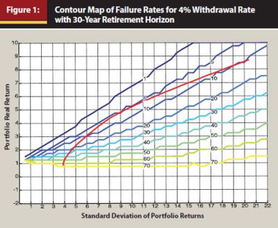
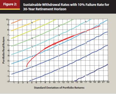
Figure 2 provides a different perspective by showing how sustainable withdrawal rates relate to the expectations about portfolio returns and risks when the failure rate is set at 10 percent and the retirement duration is set at 30 years. Here we can see, naturally, that sustainable withdrawal rates increase as returns increase or as volatilities decrease. We can also observe the offsetting relationships between returns and standard deviations in order to maintain the same withdrawal rate. Again, the efficient frontier generated from the historical data is added to this figure. In addition, the asset allocation that maximizes the sustainable withdrawal rate is identified with a circle. The MWR with a 10 percent failure rate is 4.3 percent. In addition to the optimal asset allocation, the range of points on the efficient frontier (representing a range of asset allocations) that allows for a withdrawal rate within 0.1 percentage points of the maximum is highlighted with a thicker red line. But what is the optimal asset allocation and the range of asset allocations performing nearly as well?
These answers are provided in Table 3 for a wide variety of retirement durations and failure rates. For the case just discussed, the MWR of 4.3 percent is supported with a portfolio of 45 percent stocks and 55 percent bonds. Stock allocations that provide nearly as large a withdrawal rate range from 28 percent to 69 percent. Table 3 demonstrates, unsurprisingly, that sustainable withdrawal rates are higher both for shorter retirement durations and for higher allowable failure probabilities. As well, the optimal stock allocation tends to increase both for longer retirement durations and for higher allowed failure probabilities. There is often a wide range of asset allocations that support nearly as high withdrawal rates as the optimal allocation. This table provides clear evidence of the viability of lower stock allocations to compete with higher stock allocations in retiree portfolios, even when the results are based on the excellent performance of stocks found in the U.S. historical record.
Sensitivity Analysis for Capital Market Expectations
This section describes the sensitivity of sustainable withdrawal rates to changes in some characteristics of the underlying portfolio while holding other characteristics the same as in Table 1. To provide a consistent example, these scenarios assume a 10 percent accepted failure rate and a 30-year retirement horizon, except for the cases in which these specific characteristics are modified. Readers can find visual representation of what is being described in this section by referring to Pfau (2011) online at http://wpfau.blogspot.com/2011/08/swr.html. Also note that Pfau (2011) provides additional figures showing the sustainable withdrawal rates based on returns and standard deviations for different retirement durations and failure rates, allowing readers to consider how this framework may apply to a wide variety of situations.
In the first scenario, real stock arithmetic averages are modified to take values between 4.5 and 10 percent compared with the historical average of 8.7 percent. Not surprisingly, increasing stock returns support a higher withdrawal rate for a given failure rate, and the optimal stock allocation tends to increase as well. Even if real stock returns could average 10 percent, though, the historical volatility of stocks is sufficiently high that a 5 percent withdrawal rate cannot be sustained. Holding the other portfolio characteristics constant, a 4 percent withdrawal rate cannot be sustained with a 10 percent failure rate unless real stock returns are at least 7.5 percent. With 7.5 percent returns, the optimal stock allocation falls to about 35 percent, with similarly performing allocations ranging between about 20 percent and 47 percent. If stock returns are expected to be lower, it is important to reduce the stock allocation in order to avoid an even bigger drop in sustainable withdrawal rates, suggesting that planners concerned that forward-looking stock returns will fall behind past averages would have good justification to recommend reduced stock allocations.
Another scenario keeps the real stock return at 8.7 percent, but varies the stock volatility from between 12 percent and 22 percent compared with the historical 20.39 percent. Higher volatilities reduce the sustainable withdrawal rate and the stock allocation. In this case, the optimal stock allocation can change rapidly, as the optimal allocation increases from about 60 percent to 90 percent when the standard deviation declines from 18 percent to 16 percent. A decline in volatility to about 15 percent for stocks, holding other characteristics the same, would help push the MWR to more than 5 percent and would call for a stock allocation of more than 90 percent. Meanwhile, if stock volatility nudges up to 22 percent, the MWR falls to about 4.2 percent, and the optimal stock allocation is less than 40 percent.
A third scenario considers the combined effects of the return and volatility assumptions for stocks. I consider the impact of reducing stock returns by 30 percent to 6.1 percent, reducing the standard deviation by 30 percent to 14.3 percent, and reducing both factors simultaneously by 30 percent. This is important because even when one expects lower future stock returns, the question remains about what to assume for volatility. Would lower returns be accompanied by lower volatility, or is it more reasonable to keep volatility the same? If returns drop but volatility stays the same, the withdrawal rate is pushed below 4 percent, and the optimal stock allocation falls to about 20 percent. At the same time, if only the standard deviation decreases, then the withdrawal rate increases to more than 5 percent, supported by stock allocations of at least 60 percent. However, if both factors fall so that their ratio stays the same, the overall impact is minimal. Sustainable withdrawal rates drop slightly by about 0.1 percentage point, and asset allocation recommendations stay about the same.
I next investigate the role of correlations. In the historical data, stocks experience a correlation of about 0.1 with bonds and bills. When considering the effect of changing both correlations simultaneously to various values, I find that the lower the correlation, the larger are the diversification benefits and the higher are the withdrawal rates. As correlations increase, withdrawal rates decline, and stock allocations increase, because they offer larger potential returns, and there are fewer benefits from owning fixed income. Holding other characteristics the same, with high correlations the MWR falls below 4 percent.
I also observe that increasing the retirement duration results in reductions to sustainable withdrawal rates, and a slight trend toward increasing stock allocations. A 35 percent stock allocation falls within the range of “nearly optimal” allocations for all of these retirement durations between 10 and 40 years, though. Choosing the appropriate retirement duration is very important, as longer planning horizons call for smaller withdrawal rates.
Consider a retiree planning for a 20-year retirement duration. Findings suggest that a 5.7 percent withdrawal rate can be supported with a 10 percent failure probability with a stock allocation of about 40 percent. But if the planner misjudged the client’s life span and the client lived for 30 years, the probability of failure for the withdrawal rate strategy increases dramatically to about 50 percent. If such a withdrawal rate were used, the best stock allocation would have been about 90 percent, but this still leaves a failure rate of 30 percent.
Finally, we look at the impact of fees, which could also be interpreted as portfolio underperformance against the benchmark indices. Findings show that asset allocation is not affected much by fees that affect each asset equally. In addition, fees reduce sustainable withdrawal rates, as a 3 percent fee reduces the MWR from 4.3 percent to 2.9 percent. Despite common misconceptions, there is not a one-to-one trade-off between fees and withdrawal rates. As the portfolio decreases in size, fee amounts decline, and real withdrawal amounts do not change.
Putting It All Together
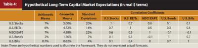
This framework can be used to estimate sustainable withdrawal rates for a given failure rate and retirement duration for almost any kind of capital market expectations. The purpose is to demonstrate how planners can translate their own expectations into an understanding about how to choose a withdrawal rate and asset allocation strategy for their retired clients. Planners could help their clients choose suitable asset classes and develop expectations about the returns, standard deviations, and correlations among the asset classes. Table 4 provides a set of hypothetical expectations for real returns in U.S. dollars for five different asset classes.
This information can then be input into a mean-variance optimizer to find the efficient frontier of asset allocations that provide the most return for a given risk or the most risk for a given return. The efficient frontier can then be plotted on the grid framework relating withdrawal rates to returns and volatilities for an acceptable failure probability and retirement duration. From this overlay, we determine where the efficient frontier reaches the highest withdrawal rate.
Returning to the mean-variance optimization results, we find the asset allocation corresponding to this optimal point. The optimal asset allocation can then be compared to the client’s investment constraints and risk tolerance to determine its acceptability. If not acceptable, other points on the efficient frontier that support progressively lower withdrawal rates can be investigated until a suitable asset allocation is found.
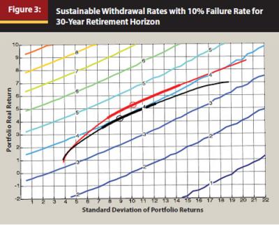
Figure 3 shows the efficient frontier with these Table 4 assumptions in black along with the efficient frontier for the Table 1 historical data in red. For this particular hypothetical example, the asset allocation that supports the highest withdrawal rate over 30 years with a 10 percent failure rate is 12.5 percent U.S. stocks, 16.7 percent U.S. REITs, 18.4 percent international stocks, 52.4 percent U.S. bonds, and no Treasury bills. This asset allocation supports a 4.0 percent withdrawal rate. If deemed acceptable, this could serve as the client’s withdrawal rate and asset allocation strategy.
Conclusion
Sustainable retirement withdrawal rates depend on capital market expectations, retirement durations, asset allocations, and acceptable failure probabilities. This article attempts to combine these aspects to provide a more complete framework for understanding the relationships between these factors. Planners can use this framework to translate their own forecasts for capital markets into withdrawal rate and asset allocation recommendations for clients.
References
Athavale, Manoj, and Joseph M. Goebel. 2011. “A Safer Safe Withdrawal Rate Using Various Return Distributions.” Journal of Financial Planning 24, 7 (July): 36–43.
Bengen, William P. 1994. “Determining Withdrawal Rates Using Historical Data.” Journal of Financial Planning 7, 4 (October): 171–180.
Bengen, William P. 1996. “Asset Allocation for a Lifetime.” Journal of Financial Planning 9, 4 (August): 58–67.
Blanchett, David M., and Brian C. Blanchett. 2008. “Data Dependence and Sustainable Real Withdrawal Rates.” Journal of Financial Planning 21, 9 (September): 70–85.
Cooley, Philip L., Carl M. Hubbard, and Daniel T. Walz. 1998. “Retirement Spending: Choosing a Sustainable Withdrawal Rate.” Journal of the American Association of Individual Investors 20, 2 (February): 16–21.
Cooley, Philip L., Carl M. Hubbard, and Daniel T. Walz. 2011. “Portfolio Success Rates: Where to Draw the Line.” Journal of Financial Planning 24, 4 (April): 48–60.
Huebscher, Robert. 2011. “The Simplest, Safest Withdrawal Rate.” Advisor Perspectives (August 23).
Milevsky, Moshe A., and Anna Abaimova. 2006. “Risk Management During Retirement.” In Retirement Income Redesigned: Master Plans for Distribution, eds. Harold Evensky and Deena B. Katz. New York: Bloomberg Press.
Pfau, Wade D. 2011. “Capital Market Expectations, Asset Allocation, and Safe Withdrawal Rates: Additional Results.” Pensions, Retirement Planning, and Economics blog (August 24). http://wpfau.blogspot.com/2011/08/swr.html.
Saltzman, Cynthia. 2006. “Balancing Mortality and Modeling Risk.” In Retirement Income Redesigned: Master Plans for Distribution, eds. Harold Evensky and Deena B. Katz. New York: Bloomberg Press.
Spitzer, John, Jeffrey Strieter, and Sandeep Singh. 2007. “Guidelines for Withdrawal Rates and Portfolio Safety During Retirement.” Journal of Financial Planning 20, 10 (October): 52–59.
Van Harlow, W. 2011. “Optimal Asset Allocation in Retirement: A Downside Risk Perspective.” Putnam Institute Retirement paper series (June): 1–15.
Williams, Duncan, and Michael Finke. 2011. “Determining Optimal Withdrawal Rates: An Economic Approach.” Retirement Management Journal 1, 2 (Fall): 35–46.