Faster Detection of Trend Changes in Slow-Timing the Market

Journal of Financial Planning: February 2014

 

 

D. Allen Cohen, Ph.D., is a senior analyst at OptiFour Integrated Wealth Management LLC in McLean, Virginia. He is a former U.S. Air Force captain and performed military operations analysis for 35 years. He was chief scientist of several military-oriented corporations and CEO and co-owner of an analytical consulting firm in Northern Virginia. He received a Ph.D. in theoretical physics from Case Institute in Cleveland, Ohio. Email D. Allen Cohen.

Kenneth D. Cliffer, Ph.D., is a senior program analyst in the U.S. Department of Health and Human Services. He received a Ph.D. in anatomy, with research in neuroscience, from the University of Minnesota. He has worked as a research scientist, as well as in developing curriculum and educational videos. Email Kenneth Cliffer.

Executive Summary

• This paper presents a “market slow-timing” portfolio allocation strategy based on anticipation of the market generally moving up or down over intermediate-duration periods. This approach differs from other “market timing” practices.
• Market slow-timing is based on bullish and bearish stock-market statistical trends as described by Cohen (2011a). The approach uses the historical monthly closing values of the S&P 500 Index and the Consumer Price Index, starting in 1901. Since 1901, 24 bullish-to-bearish and 24 bearish-to-bullish transitions have occurred between trends ranging in duration from seven to 114 months.
• As distinct from other practices of market timing, market slow-timing is based on using an analytical algorithm to identify trends of monthly percentage market changes that are statistically biased to be more likely to go upward (bullish) or downward (bearish). These trends last sufficiently long that client portfolio reallocations near a trend’s identifiable beginning have been shown to be financially advantageous for the client.
• Projected results from an example application, using an in-house financial planning model, reflect the advantage of appropriate allocations earlier during new trends using a new detection method. Depending on the criterion, median results showed increases in average annual yield of invested assets from 5.3 percent for a conventional approach, to between 5.5 percent and 6.3 percent for the described approach.

Acknowledgement: The authors thank OptiFour Integrated Wealth Management LLC for supporting this research, in particular, OptiFour founding partner I. Mark Cohen, J.D., LL.M., CFP^®. The views expressed herein are those of the authors individually, and are not to be taken as representing positions or views of OptiFour Integrated Wealth Management, the U.S. Department of Health and Human Services, or the United States.

Stock market bullish and bearish statistical trends,¹ which can be useful for adapting client portfolio allocations, can be identified using a spreadsheet procedure for “slow-timing” the market (Cohen 2011a). The historical durations of these intermediate-duration trends over the past 112 years have ranged from seven months to 114 months. One drawback of the procedure previously presented by Cohen is that a trend change may take six to eight months after the transition to be identified, at which time the new trend is already in progress. However, even with this drawback, reallocating one’s securities portfolio to be more aggressive during bullish trends and more defensive during bearish trends has been demonstrated to be generally advantageous.

The impetus for developing the slow-timing approach to asset allocation resulted from financial planning clients who were frustrated with the prevalent strategy of persistently maintaining existing allocations during recessions and riding them out. However, financial planners tend to be justifiably wary of “market timing” (Hulbert 2013).² A potential solution would be to identify statistical trends with durations sufficiently long to afford reallocating portfolios advantageously while not being so long as to be impractical. These are designated “intermediate-duration” trends.

The idea that such intermediate-duration statistical trends can be identified in stock market behavior came from Mandelbrot’s (1997) insight and demonstration that the temporal behavior of stocks is essentially fractal. The trends, as identified here, are not the same as conventionally defined primary bull and bear markets. Beginnings and ends of primary market trends are identifiable only after a 20 percent market change in one direction and then the other (Browning 2008). A primary bull or bear trend can be as short as one month for a rapid change that then reverses. In addition, because a primary market trend is not recognized until the 20 percent threshold is reached, the start of a slow trend (and simultaneously the end of the previous trend) may take a long time to recognize.

In contrast, as described later, the slow-timing approach allows consistent recognition of changes in intermediate-duration trends within eight months and, with the approach described here, detection in an average of about two to three months, and always within five months. The approach is not dependent on large-magnitude overall changes, but rather on a limited set of changes reaching a defined threshold at the beginning of a new trend. This new trend continues until the threshold of changes in the opposite direction is reached. In addition, the underlying market statistics on which the approach is based, as demonstrated and discussed later in this paper, have been remarkably consistent. In contrast, judgments regarding when bull and bear primary trends have begun—before they have fully developed—have been remarkably inconsistent (Hulbert 2013).³

An algorithmic procedure was developed by Cohen (2011a) to identify intermediate-duration trends⁴, a procedure designated the “algorithmic-recognition” approach (“recognition” for short). This algorithm is presented mathematically in Appendix A (found online at FPAJournal.org). It operates on a market attribute that describes market behavior: the trailing, 12-month running average of the S&P 500 Index (first-of-the-month values), normalized relative to inflation to the December 1902 dollar value. (In this paper, the S&P 500 refers to the price return S&P 500 Index, which has the index symbol SPX.) The procedure uses the month-to-month percentage change of this average, the latest currently determinable change (“latest change”) from the prior month, and the successive sums of that latest change plus up to five prior monthly percentage changes.⁵

When the latest change or one of the sums reaches or exceeds a predetermined threshold, a trend transition is recognized. The transition month is the earliest month figuring in a calculation contributing to the threshold-reaching sum.⁶ The month when the recognition occurs is called the “recognition month.” A threshold value of 3 percent (bearish-to-bullish) or –3 percent (bullish-to-bearish) was experimentally determined to result in trends of durations appropriate for financial planning purposes (months to years). Because the latest value of the Consumer Price Index (CPI), which is used to calculate the inflation-normalized values, becomes available at the beginning of the second month following that to which it applies, the latest currently determinable change is that for two months prior to the current month.

The algorithm was developed heuristically by testing numerous candidates. Each candidate algorithm was applied month-by-month to the historical monthly values of the S&P 500 as adjusted by the CPI (both of which are required by the algorithm) starting in January 1901⁷ and continuing through February 2013. For the formulation of the algorithm, the S&P 500 was chosen because it has maintained its relevance to the breadth of the securities market, is universally accepted, dates back to the beginning of the 20th century, and is readily accessible. To allow the algorithm to use constant-dollar values of the S&P 500, the CPI is used to remove the effects of inflation, as CPI values are readily available back to the beginning of the 20th century. The 12-month trailing average of the constant-dollar S&P 500 dampens out short-term market fluctuations such that the algorithm addresses the targeted, more fundamental, intermediate-duration statistical trends.

Cohen (2011a, b) established three key aspects of the utility of this method: (1) the resulting statistical distributions of historical intermediate-duration bullish and bearish trends as determined by the algorithm are valid statistical trends; (2) even given the trend-transition-recognition lag time, the application of these trends to portfolio reallocations (with their attendant costs) is generally advantageous to the client; and (3) the algorithm can be applied by financial planners.⁸

The algorithmically derived historical trends are displayed in Figure 1.

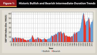
In Figure 1, one can readily see that blue (bullish) segments generally go up, while red (bearish) segments generally go down. One can also get a sense of the variation in ­trend-segment durations. As of July 1, 2013, the stock market was beginning the 48^th month of the then-current bullish-trend period

The Statistical Detection Procedure

The key to identifying trend changes earlier, as they are occurring, is to use the historical statistical distributions as indicating probabilities of monthly percentage changes, to project the likelihood of different courses of the market in the near-future months.

The recognition procedure (Cohen 2011a) is retrospective. It looks back to determine if a trend transition already has taken place. The detection
procedure described here uses a projection algorithm to look ahead. It uses these projections to estimate the likelihood of a trend change being currently underway. The likelihood is based on the past behavior of the S&P 500 under similar circumstances. Even though the past does not necessarily portend the future, it often is the best available source of insight; the historical stability of the frequency distributions used to indicate probabilities for the projections (see Appendix B below) provides confidence in the utility of the approach.

The statistical distributions at the foundation of the method to identify the trends earlier are the cumulative frequencies of the month-to-month percentage changes of the S&P 500 (not normalized to December 1902 dollars), and of the CPI, separately tabulated for bullish and bearish periods, and applied as cumulative probability distributions. The distribution for the S&P 500 is illustrated in the online Appendix B, along with evidence that it has been historically stable over the course of the last century, despite great changes in specific historical influences.

The projections used to detect trend changes earlier than can be accomplished with the recognition method are Monte Carlo projections of the index values forward in time. Monte Carlo projections use probability distributions to develop successive, computer-generated trial projections in which the likelihood of outcomes is governed by the distributions.⁹ Many financial planning computer models use this type of Monte Carlo process to project probabilities of future outcomes. However, to our knowledge, no such model incorporates bullish and bearish trends. Near-term projections of the S&P 500 and the CPI are part of the statistical-detection process presented here.

One also can incorporate bullish and bearish trends in extended market projections to project investment performance, as is incorporated into estate projections described later in this paper. To do this, besides accounting for distributions of monthly changes in the indices as previously described, one also must account for trend durations, which can be done using the statistical distributions of trend durations (see Appendix B).

For each run¹⁰ for extended projections of future market behavior, the Monte Carlo process is first applied to determine a sequence of trend durations (using the smoothed versions of the cumulative-frequency duration profiles in online Appendix B, Figure B2): bullish, bearish, etc.; this procedure thereby determines the transition dates for the run, considering historical frequencies as probabilities. For extended projections and for near-term trend-detection projections, the Monte Carlo projection process is applied to determine projected monthly changes in the S&P 500 and in the CPI using the appropriate cumulative-frequency curves (see online Appendix B, Figure B1 for the S&P 500; not shown for the CPI), separately for bullish and bearish periods, as indicating probabilities. In this way, each run reflects values of the S&P 500 and of the CPI appropriately for both bullish and bearish trends and appropriate durations of trends for extended projections. Such Monte Carlo projections of the S&P 500 and the CPI are used in the statistical-detection procedure, as described below, using statistics for the trend opposite the currently recognized trend.

The algorithmic-recognition procedure was previously used for recognizing, in the “recognition month,” that a trend transition had occurred in a month, the “transition month,” up to eight months earlier. The eight months is accounted for by the up-to-six months of monthly changes contributing to the sums of monthly changes plus the two-month lag in obtaining the CPI to get the latest determinable month’s inflation-adjusted S&P 500 Index value. The “statistical-detection procedure” described here uses the recognition procedure applied (month-to-month) using the forward Monte Carlo projections of the two indices: the S&P 500 and the CPI.

The monthly values of the two indices are projected forward in time from their most recent reported actual monthly values to six months into the future. This is six months projection for the S&P 500, for which the most recent actual value is that of the current month, and eight months projection for the CPI, for which the most recent actual value is for two months ago (the CPI month). Thus, CPI projections include values for the current and previous month, as well as into the future. To provide an adequately great number for statistical inference, 5,000 sets of such projections (runs) are made. Then, for each run the recognition procedure is applied to determine whether any month for which projections were made would constitute a projected recognition month for that run, recognizing a transition month up to six months earlier.

Collectively, the 5,000 runs permit estimation of the probabilities that any of the projected months going up to six months into the future will recognize a transition. The estimated probabilities are the percentages of runs (of the 5,000) having affirmative results for the given month from the recognition algorithm.¹¹ A result that all or nearly all of the runs fail to result in a recognized transition in the projected months indicates a probability near zero that a transition is near. This is the case for 4/1/2009, as shown in Table 1.

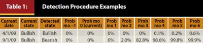
On the other hand, as shown for 9/1/2009, a result in which close to 100 percent of the runs result in a recognized transition in one or more of the projected months indicates that the current month is likely in the near vicinity of a trend-transition month. A transition near 9/1/2009 was later identified by the recognition method as occurring in August 2009.

In Table 1, the months for which probabilities are tabulated are relative to the current month at the time of the detection being simulated, so that month 0 is the then-current month (the latest month for which S&P 500 data is available), and month –1 is the first month for which the CPI is projected, which is one month prior to the then-current month and one month after the date for which the latest CPI data is available.

Assessing Detection Criteria

Historical data have been used to establish criteria for “statistical detection” for the purpose of making timely allocation changes. Applying the procedure with candidate criteria to historical data results in detection, in the “detection month,” between three months prior and five months after the month of transition. Portfolio allocation changes should be made upon detection of the transition, in the detection month, to be as close as possible to the actual transition.

The statistical-detection procedure was applied as though it were done each month from February 1, 1902, to February 1, 2013. For each application, a sequence of projected monthly probabilities was recorded (similar to Table 1). Also recorded were the historical trend-transition months and the recognition months.

To determine an effective criterion for applying the detection method, each month’s projected probability of a transition being near (Prob mo –1 through Prob mo 6) was tabulated. The goal was to set a threshold value as a criterion that would minimize the number of false alarms or missed detections while providing an early detection of a transition. A detection is indicated by any of the monthly probabilities reaching the criterion’s threshold value. Once recognition occurs, which definitively indicates the transition month, one can determine when the statistical detection occurred relative to the transition month.¹²

Statistics collected on the results of applying each candidate criterion to all of the historical dates were the nearness of the detection month to a transition month and the number of (1) false alarms or (2) missed detections of each type. Criteria were evaluated of at least a 60 percent, 75 percent, or 90 percent probability in any of the projected months of a recognition: “D-60 percent,” “D-75 percent,” and “D-90 percent” detection (“D”) criteria, respectively. In no case did the application of any of these criteria result in missing a transition. False alarms indicated transitions when none were near. The D-90 percent criterion did not result in false alarms, but the D-75 percent and D-60 percent criteria did.

In all cases in which the D-75 percent and D-60 percent criteria indicated detections near actual transitions, the D-90 percent criterion indicated a detection within four subsequent months. Based on this finding, a secondary criterion of D-90 percent detection within four subsequent months was set to confirm a detection with the D-75 percent or D-60 percent criteria. For example, if the D-60 percent criterion indicated a detection, which would signal the appropriateness of an allocation change, the lack of a confirmation D-90 percent criterion being reached within four subsequent months would then indicate that the D-60 percent criterion had yielded a false alarm. A change in allocation stimulated by the false alarm could then be rectified by reverting back to the original allocation.¹³

Table 2 summarizes key aspects of the projections for the 48 historical trends, the recognition and detection (using the candidate criteria) of trend transitions, the durations of the trends, indications of false alarms, and summary statistics. The table includes summaries of the numbers of months that deviations of allocation strategies from the existing trends would have been present historically if the various recognition and detection criteria had been used. Negative values in Table 2 indicate detection of a transition prior to its occurrence. The summary portion of Table 2 indicates the timing advantages of (1) the statistical detection approaches (D-x%) over the recognition approach and (2) the lower-percentage detection criteria.

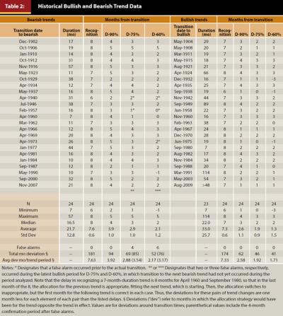
Figure 2 contains plots of the overall cumulative frequencies of transition recognition and detection in the months before and after the transition occurred. This includes plots for each of the candidate transition-detection criteria, based on the last 112 years of market behavior. It illustrates that the D-60 percent criterion results in about a 17 percent probability of a transition being detected on or before the transition month (13 percent for bullish to bearish; 21 percent for bearish to bullish [not illustrated]).

 

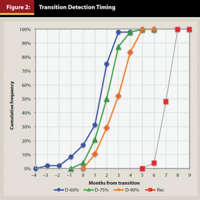
Using the D-90 percent, D-75 percent, and D-60 percent criteria, 52, 88, and 98 percent of transitions, respectively, were detected by three months after a transition. In all cases, transitions were detected by five months after they occurred. In contrast, recognition occurred six to eight months after a transition. The lower-percentage criteria detect transitions progressively earlier. This also is reflected in the average detection delays overall of 3.3, 2.4, and 1.7 months, respectively; the average delay for recognition is 7.5 months.

Table 2 also shows that trend transitions from bearish to bullish tend to be detected earlier (2.6, 1.9, 1.3 months, respectively, on average) than those from bullish to bearish (3.9, 2.9, 2.1 months, respectively). However, despite resulting in earlier detection of trend transitions, the lower-percentage criteria result in false alarms.

An advantage of the lower-percentage criteria is that trends can be responded to more quickly after transitions. A disadvantage is that portfolio changes will occasionally be made erroneously and allowed to stand for several months before correction. However, the lower-percentage criteria still result in less time in inappropriate allocations, despite the false alarms.

Analyses indicate that the trends in the market immediately following trend transitions are stronger than the general trends (see online Appendix C). This resembles the well-recognized tendency for primary bull and bear markets to start with their characteristic behaviors exaggerated. However, given the difference previously noted between the trends defined here and primary bull and bear markets, the exaggeration in intermediate-duration trends near their beginnings is a distinct phenomenon. This tendency makes the rapid detection of the trend transitions to change allocations as soon as possible especially important. Importantly for the utility of the approach described here, the market behavior remains biased (bullish or bearish) during the non-transitional periods within established trends (see online Appendix C).

Assuming an allocation change is implemented immediately upon detection of a trend change, and changed back four months later if a false alarm is indicated by failure to confirm using the D-90 percent criterion, use of the D-60 percent criterion results in the least “deviation” (“dev”) over the 112-year historical period. This pattern is shown in Table 2 separately for transitions to bearish trends and transitions to bullish trends (overall for combined data, including deviations due to false alarms: recognition: dev = 355 months total; average 7.4 per transition; D-90 percent: dev = 156 months total; average 3.3 per transition; D-75 percent: dev = 131 months total; average 2.7 per transition; D-60 percent: dev = 117 months total; average 2.4 per transition). Therefore, use of the D-60 percent criterion with confirmation by the D-90 percent criterion appears to be a particularly advantageous strategy.

However, if a client’s tolerance for false alarms and “mistaken” switches in allocation is low, a D-90 percent criterion may be a better choice. It is clearly better for quicker detection than can be achieved by the recognition approach, which takes substantially longer to recognize that a transition has occurred. The D-75 percent criterion with D-90 percent confirmation results in fewer false alarms than D-60 percent but more deviation months overall (albeit fewer than D-90 percent alone).

All of the historical would-be false alarms under the tested set of detection criteria occurred during bullish periods, falsely indicating bullish-to-bearish transitions. A false alarm is theoretically possible using any of the tabulated detection criteria, although the historical false-alarm counts of zero for the D-90 percent criterion, noted in Table 2, indicate that false alarms for this criterion are highly unlikely. When, in practice, a false alarm does occur, it signifies that the market trend came near to transitioning but did not quite make it. Historically, the greatest delay between D-90 percent detection and recognition was eight months. The greatest delay between D-75 percent or D-60 percent detection and recognition was 10 months. Therefore, one could definitively confirm or deny detections within these time frames using the recognition algorithm.

It is important to emphasize that the statistical results presented here are based on 1,346 months of data incorporating 48 historical trend transitions dating back to 1901. The following presumptions are associated with applying the statistical-detection method going forward:

1. Sequential trend durations are not strongly correlated.¹⁴
2. The market behavior as characterized here will not change substantially in the future, which is most likely if the underlying historical causal factors that have underpinned the market will continue to apply.
3. Statistical results favor the more likely events (however, singular events can have a significant influence not picked up by statistical projections).

Many underlying historical factors influence market behavior, including the world economic outlook, consumer confidence, the political environment, and the season. This is not meant to imply that the underlying influencing forces are all known and that their causal relationships to market behavior are understood. Rather, collectively over the past 112 years, these influences have gone through their many correlated variations such that a new significant influence is not likely.

However, applying the statistical distributions of the indices derived from the entire 112 years of data to that period could raise concerns about the validity of using these findings for future projections. To address this point and to address presumption 2 in the previous list, an out-of-sample test was performed in which the index statistical distributions for the first 55 years of the 20th century were applied to the 55 remaining years up to the time of testing. The resulting detailed numbers differed slightly, but the statistical-detection dates and delays matched. This equivalence is due to the temporal stability of the statistical distributions of the monthly market changes (see Appendix B with Figure B1).

Example Projected Application

Projections of estate behavior were made using extended projections of market behavior as previously described in this paper, using the statistical distributions. These projections were used to test whether relative performance of applying the various transition-detection and transition-recognition strategies would follow the previously noted inferences that successively lower-percentage criteria would result in successively better performance due to decreasing deviation from appropriate allocations.

Figure 3 presents the results of an analysis projecting financial results of an actual client’s estate using the company’s in-house model. Although projected portfolio performances depend on specific allocation strategies and client financial details, we have found these projection results to be generally typical of financial planning clients.

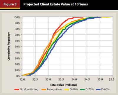
In Figure 3, cumulative frequencies of results from 300 runs are plotted, each run projecting a total estate value in 10 years of an estate initially worth $2.27 million. The strategy for no slow-timing (the red plot) was to maintain a well-diversified, moderately conservative portfolio of separately managed accounts (SMAs) throughout the 10 years. The recognition strategy (the orange plot) was to modify the portfolio allocation based on Cohen’s (2011a) method of retrospective algorithmic recognition of trend changes.

The strategies for the detection strategies (yellow, green, and blue plots) were to modify the portfolio allocation based on the statistical detection of trend changes using the D-90 percent, D-75 percent, and D-60 percent criteria, with the D-90 percent verification of trend changes for the D-75 percent and D-60 percent criteria to limit anti-trend effects of false alarms to four months. Approximately half of the estate total value participated in trend-change reallocations. Under the trend-driven allocation-change strategy, the allocation for bullish trends was chosen to favor more aggressive SMAs. For bearish trends, it favored more defensive SMAs. The model analysis included calculations of the fees and taxes incurred on making portfolio changes, as well as client-stipulated cash flows. As such, the analysis accounted for the increased expenses incurred in portfolio reallocations.

For the D-60 percent and D-75 percent strategies, false alarms were incorporated into the analysis, randomly assigned with frequencies corresponding to their historical frequencies. Thus, in any given run, one or more false alarms may or may not occur (because their historical frequencies were less than one every 10 years), even though collectively they occurred in the runs at the historical frequencies.

When a transition false alarm occurred during any statistical projection, the corresponding portfolio reallocation was performed as though it detected a real transition, as would occur using that strategy. Then, four months after the false alarm, when the D-90 percent criterion would not have confirmed the transition (according to its historical record of no false alarms), the portfolio was reallocated back to its prior state, with all of the involved fees incurred.

As anticipated from the relative numbers of months of deviation from appropriate portfolio allocations in the historical analysis previously noted, overall the plots show successively improved results for the D-90 percent, D-75 percent, and D-60 percent strategies relative to the recognition strategy. Each of the detection strategies yielded statistically significantly higher distributions of values than those of both the recognition and the no slow-timing strategies (see online Appendix D).

Although low-end results are not substantially different between no slow-timing and the recognition method, the results at the higher end of the recognition distribution clearly diverge to be higher than those of no slow-timing. Results at the higher end approach those for the detection methods. The higher end reflects runs in which the market tended overall to have fewer trend changes and longer bullish trends, resulting in fewer allocation-change fees and greater growth.

The relative opportunities and risks of using these approaches are reflected in the overall distributions of results, not those of any one location within the distributions. Nevertheless, the median results at the middles of these distributions are arguably typical results: (1) no slow-timing: $3.04 million; (2) recognition: $2.98 million; (3) D-90 percent: $3.08 million; (4) D-75 percent: $3.11 million; and (5)D-60 percent: $3.23 million.

Considering only the part of the estate value participating in the reallocations (about half), the average annual growth rates of the participating investments in the median runs were 5.3 percent, 5.0 percent, 5.5 percent, 5.7 percent, and 6.3 percent for the five approaches, respectively. The percentage differences in these average annual growth rates at the median projections for the recognition, D-90 percent, D-75 percent, and D-60 percent approaches compared with that for the conventional approach were –7.1 percent, +3.6 percent, +7.2 percent, and +18.3 percent, respectively.

Commentary, Issues, and Recommendations

The results show the advantage of the statistical-detection slow-timing method over the initially described recognition slow-timing method, which itself shows an advantage at the high end of the distribution over that of conventional portfolio allocation approaches. Remaining issues include (1) how to interpret the results; (2) how much faith to put into the results; and (3) what action strategies would be beneficial for financial planning clients. Before discussing these issues, consider first the role of the past and its characterization in plotting a future course.

Financial planners develop intuitive insights informed largely by their experiences. Depending on the breadth and depth of those experiences, planners will each interpret the past and present market behaviors with subconscious biases that tend to favor one interpretive, predictive approach or another, such as rules of thumb, pattern charting, or Monte Carlo statistics. All approaches are based on historical market behavior. None are foolproof, given that the past does not necessarily predict the future.

Taleb (2010) coined the term “black swan” to describe statistical outlier events that are unique, unpredictable, and strongly influential. He made the case that the principal advancements in human fields of endeavor are by virtue of black swans, notwithstanding statistical and other future-projection approaches. So, if Taleb’s basic premises are accepted, where does this leave statistical, historical approaches, including the ones presented here?

We submit that Taleb’s premises are not entirely applicable to this line of research. The approach presented in this paper (1) uses actual statistical distributions based on all the available historical data and not some analytical approximation or theoretical construct, and (2) includes historical time periods during which market-related black swans did occur. The analysis thus does not ignore past statistical outliers. Nevertheless, by definition, future black swans will not be predicted, nor their probable occurrences projected by this or any other technique. Therefore, no approach can prospectively account for these outlier events. However, should a black swan occur, subsequent analyses will benefit from and eventually account for the impacts of the black swan. In this manner, statistically projecting market behavior remains dynamic.

Acknowledging the possibility of statistical anomalies, how should a financial planner interpret the model’s results? When all of the projected months’ probability values for a trend transition are near zero, the near-term months are unlikely to be trend-transition months. When the maximum projected probability value relative to the current month is equal to or greater than the selected detection criterion, a trend-transition month is likely to be near the current month, and highly likely to be within four months (see Figure 3).

How much faith should a planner put into the results? These results can be considered reasonably reliable in that they are based on 1,346 months of historical data. However, black swans will inevitably occur. Nevertheless, no method can account for these before they occur.

What action strategies would be most beneficial for financial planning clients? Regarding which detection criteria to use, as a single criterion and considering historical false alarms, the D-90 percent criterion is more conservative than the D-75 percent criterion, which is more conservative than the D-60 percent criterion. Importantly, however, the lower-percent criteria generally detect trend transitions progressively more quickly, with correspondingly better results. Also, historically, the detections of transitions from bearish-to-bullish trends have not exhibited false alarms.

Given the above considerations, the approach of using the D-60 percent criterion in conjunction with confirming (or denying) its detections with the D-90 percent criterion provides the best way to balance the rapidity of detection from the lower-percent criterion while correcting relatively quickly for false alarms. This combination approach is supported by its providing the fewest months of off-trend investment in the historical application and by the example results. If transaction charges for making and correcting false alarms are of high concern, one could use the D-75 percent criterion with correction using the D-90 percent criterion, at a cost of somewhat slower detection of trends.

In general, no prescription should be followed blindly. Ultimately, a planner’s overall judgment should and will prevail, because the planner is most attuned to the client’s needs and disposition. Having said that, the authors’ judgment is that these results are sufficiently reliable for the planner to assume their validity when deciding what action, if any, to recommend to clients.

For ONLINE ONLY APPENDICES, please click HERE.

Endnotes

1. A statistical trend refers to a series of non-random changes. These are changes biased to be more likely to be up during some (“bullish”) periods or down during others (“bearish”).
2. Hulbert (2013) noted, “Even those who do beat a buy-and-hold strategy in one market cycle have no greater odds of success in the next cycle.”
3. Hulbert (2013) noted that Bob Brinker, who had provided timely and effective advice regarding the 2000 and 2003 changes in the market, indicated that his failure to do the same for the 2007–2009 bear market was “because it was historically unique—‘a once-in-a-lifetime financial train wreck.’” In contrast, as shown in Table 2, a 21-month bearish trend that started in November 2007 would have been detected using the approach described in this paper between January and March 2008, whereas the primary bear market trend was not recognized until late June 2008 (Browning 2008). Even using the original recognition approach for slow-timing, the recognition would have been made at the beginning of July 2008 (eight months after the beginning of the trend), about the same time as the recognition of the primary bear market trend.
4. The analysis presented here updates that in the previous paper (Cohen 2011a) with more recent market values as well as technical improvements; the main approach, results, and conclusions have not changed.
5. The sums include (1) the latest change plus the prior month’s change; (2) the latest change plus the sum of the two prior months’ changes; and so on up to (5) the latest change plus the sum of the five prior months’ changes.
6. Because a change is the difference between a given month and the previous month, the earliest month figuring in such a calculation is the month prior to the earliest one for which a change (from that prior month) contributes to the calculation. When recognition is made for less than the full six-month span tested, and a threshold calculation in a subsequent month indicates a transition earlier, the earlier date is taken as the actual transition.
7. Adjustments for inflation start for January 1903, converting to December 1902 dollars.
8. Cohen (2011b), an FPA Virtual Learning Center webinar, presented the formulation of this algorithm programmed in a Microsoft Excel worksheet so participants could develop their own worksheets.
9. Referring to the bullish curve of Figure B1 in Appendix B, the Monte Carlo process begins by drawing a random number between 0 and 100, say, rand = 65.5. From the bullish curve, the 65.5 percentile value (ordinate) corresponds to a 2.53 percent monthly change (abscissa) in projecting the value of the S&P 500 forward to the next month; i.e., next-month’s index value = prior-month’s index value * (1+(2.53/100)). This is done repeatedly month-to-month for as far forward into the future as desired. One such projection by itself has little value; however, a great number of such projections gives insight on the range of future possibilities and their likelihoods of happening, presuming the future behaves statistically like the past.
10. A “run” is the sequential Monte Carlo projection forward of the index for a prescribed number of months.
11. Due to using the trailing 12-month average of the S&P 500 in the recognition procedure, by the time that a new trend can be recognized, the market will have been in that trend for some time. To account for this in the detection procedure, the projection forward of the indices use the statistics for the trend that the method is designed to detect, which is the trend opposite to the one that is currently recognized. Given the delay of six to eight months in recognizing a new trend, the detection procedure cannot be used for the next-following trend until the new trend has been underway for six to eight months.
12. The transition to a bearish trend in November 2007 noted in Table 2 deserves comment. Whereas the algorithmic recognition delay was eight months (recognized July 1, 2008), the statistical detection with the 90 percent criterion (D-90%) occurred on March 1, 2008, four months after the transition month, and detection with the lower-percent criteria (D-75% and D-60%) occurred two months prior to that. These detections would have indicated a time to become more portfolio defensive. The market remained in general decline over the following months. Then, between October 1, 2008 and November 1, 2008, the S&P 500 dropped some 200 points, signaling the beginning of the Great Recession.
13. Although a D-90 percent confirmation occurred within four months of a D-75 percent or D-60 percent determination in every case in which an actual transition was in the vicinity of the D-75 percent or D-60 percent determination, a failure of the D-90 percent confirmation is a possibility. Monitoring for a late D-90 percent confirmation and application of the recognition approach could prevent perpetuation of a false-alarm-based allocation for any more than 10 months.
14. The correlation between 46 historical trend durations and the subsequent trend durations is –0.04. Considering bullish and bearish durations separately, for 23 bullish durations and the subsequent bearish durations the correlation is 0.18, and for 23 bearish durations and the subsequent bullish durations the correlation is –0.09. None of these correlations is statistically significant.

References

Browning, E.S. 2008. “Dow Hits Bear-Market Territory, Signaling Woe for Economy.” The Wall Street Journal, Leader Section, June 28.

Cohen, D. Allen. 2011a. “Slow-Timing the Market, an Alternative Portfolio-Allocation Approach.” Journal of Financial Planning 24 (2): 45–53.

Cohen, D. Allen. 2011b. “Slow-Timing the Market.” FPA Virtual Learning Center webinar, March 2.

Hulbert, Mark. 2013. “Can Market Timers Beat the Index?” The Wall Street Journal, Weekend Investor section, July 19.

Mandelbrot, Benoit B. 1997. Fractals and Scaling in Finance: Discontinuity and Concentration. New York, New York: Springer-Verlag.

Taleb, Nassim N. 2010. The Black Swan: The Impact of the Highly Improbable. New York, New York: Random House.

Citation

D. Allen Cohen, and Kenneth D. Cliffer. 2014. “Faster Detection of Trend Changes in Slow-Timing the Market.” Journal of Financial Planning 27 (2): 50–59.