Journal of Financial Planning: August 2021
Executive Summary
- Client-specific information can and should result in significantly different forecasted retirement periods.
- After a review of assumptions used in 31,211 financial plans in Canada, retirement end age assumptions do not appear to be very personalized, given the prevalence of certain end ages, especially those that are a multiple of five (for example, approximately 70 percent of plans used age 90, and 20 percent of plans used age 95).
- Assumptions used by financial advisers also did not appear to incorporate the additional “tail risk” associated with the longer potential retirement period for a married couple.
- The length of retirement in a financial plan should be determined considering the shortfall aversion metric (for example, probability of success) to ensure recommendations are not overly conservative.
- Adding five years to projected life expectancy for a single household and eight years to the longest life expectancy of either member of a joint household (or to each member if separate end ages are used), at retirement, is an appropriate retirement end age assumption if the outcome variable is the probability of success (using a Monte Carlo model) and only fixed periods can be modeled (mortality rates are not directly incorporated). This approach suggests a retirement period of 30 years (to age 95) is a reasonable assumption for the average 65-year-old male/female couple retiring today.
- Retirement period assumptions should be revisited regularly to ensure they are timely, similar to other key assumptions in a financial plan.
David M. Blanchett, Ph.D., CFP®, CFA, is the head of Retirement Research, DC Solutions at QMA, a division of PGIM, and an adjunct professor of wealth management at the American College of Financial Services. He is the recipient of the Journal’s 2007 Financial Frontiers Award and its 2014, 2015, and 2019 Montgomery-Warschauer Award.
NOTE: Click on images below for PDF versions.
JOIN THE DISCUSSION: Discuss this article with fellow FPA Members through FPA's Knowledge Circles.
FEEDBACK: If you have any questions or comments on this article, please contact the editor HERE.
Financial plans require a significant number of assumptions. One of the most important assumptions is how long retirement lasts. This paper explores various factors relating to how to estimate “the end” of retirement in a financial plan.
In theory, retirement periods should be personalized for each client in a financial plan, based on that client’s facts and circumstances, considering various attributes such as years until retirement, income, health status, smoker status, and so on. However, a review of the key assumptions in 31,211 financial plans in Canada suggests financial planners are likely not personalizing mortality assumptions, given the predominant use of certain ages and the focus on using periods in multiples of five—approximately 70 percent of assumed retirement end ages are age 90, and 20 percent of end ages are age 95.
Given the data above, it appears that—at least for those using that particular software—there is no consensus on the approach to estimating the length of retirement among financial planners, even if the decision is based on the same underlying mortality rates (or life tables). Some planners are going to use more conservative assumptions than others for a variety of reasons.
The projected length of retirement should be determined in conjunction with the shortfall aversion metric (for example, probability of success). Mortality is a variable that is not commonly randomized in a financial plan (for example, in a Monte Carlo setting), and assuming retirement is a fixed period and estimating required savings (or available spending) based on a target probability of success can potentially result in inaccurate forecasts regarding the success of a given strategy (Blanchett and Blanchett 2008).
Through simulations, it is determined that adding five years to the life expectancy estimate for a single household and eight years to the longest life expectancy of either member of a joint household (or to each member if separate end ages are used for spouses), at the assumed retirement age, is a reasonable approach to approximating the retirement period, assuming the outcome variable is the probability of success (using a Monte Carlo model) and only fixed periods can be modeled (mortality rates are not directly incorporated). While more complex approaches that consider the distribution of mortality would be more robust, such as modeling survival stochastically, these techniques are uncommon in planning tools today. These models suggest a retirement period lasting to age 95 (that is, 30 years) would be appropriate for the average 65-year-old male/female couple retiring today.
Like any assumption in a financial plan, mortality estimates should be regularly revisited. Mortality models, along with client health, are constantly evolving, and ensuring mortality assumptions reflect all available information is an important point to consider when updating a financial plan.
In summary, forecasting “the end” of retirement is a complex decision. There is no one single “right” way to do it; however, it is important that estimates be personalized to household attributes, and that the assumed length is determined in light of other modeling assumptions, such as the probability of success, to ensure an appropriate value is selected
Estimating the Length of Retirement
The internet provides a wide variety of free tools, of varying levels of complexity, that an individual can use to estimate the potential length of retirement. Most tools provide a single life expectancy estimate based on the individual’s current age. There are two important reasons these estimates might need to be adjusted when forecasting how long retirement might last in a financial plan.
First, the retirement period should typically be determined by assuming that the probability of surviving to retirement is 100 percent. While it is certainly possible that an individual may die before retiring, this outcome should not jointly be considered when assessing how long retirement may last (and how much it may cost). Therefore, mortality estimates should be based on the age (or year) of assumed retirement, not today. This is especially important for younger individuals given the impact of improving mortality rates over time.
Second, while life expectancy is a useful metric when estimating how long someone may survive, on average, there is approximately a 50 percent probability the individual will survive beyond the period. Therefore, even if the individual has a 100 percent probability of accomplishing their retirement goal to life expectancy, the actual probability of accomplishing the retirement is not 100 percent because he or she may live longer than expected. A better approach is to consider the probability of surviving to various ages and selecting some period longer than life expectancy to ensure a cushion will exist should the individual survive longer than average. Modeling periods longer than life expectancy is especially important for couples, since they typically must plan for the longer potential retirement period of either member, which introduces additional tail risk into planning.
An example of an online tool, available for free, that provides insight into the probability distribution of survival for both an individual and a couple is the “Longevity Illustrator” tool made available by the American Academy of Actuaries and the Society of Actuaries. The tool incorporates attributes such as age at retirement, years to retirement (that is, improvement), gender, smoker status, and health when estimating mortality rates. The tool also determines the length of retirement, assuming the individual has a 100 percent probability of surviving to retirement.
The concept of survival probabilities is demonstrated in Figure 1, based on estimates obtained from the Longevity Illustrator tool. The analysis is based on an assumed couple, John (male) and Jane (female), both age 65 in average health who are nonsmokers and currently at retirement (retiring at age 65). The probabilities of survival at various ages are included for John, Jane, either member of the couple, or both members.

Survival probability provides a more comprehensive perspective on the potential duration of retirement than focusing solely on life expectancy (which is just an average). For example, the median (50 percent) survival probability, which is generally relatively close to life expectancy, is 16 years for both members, 20 years for John, 23 years for Jane, or 27 years for either member of the couple. However, there is a 25 percent probability that retirement could be 22 years, 26 years, 29 years, or 31 years, for both, John, Jane, or either, respectively. Changing the probability of survival from 50 percent to 25 percent increases the potential retirement period by about six years.
Household attributes can have a significant impact on survival probabilities and corresponding retirement period estimates. This effect is demonstrated in Table 1, which includes estimated retirement periods (in years) at various survival probabilities based on different health status levels (both members: poor, average, or excellent) and smoker status for the base couple (John and Jane). Again, all estimates are obtained from the Longevity Illustrator.
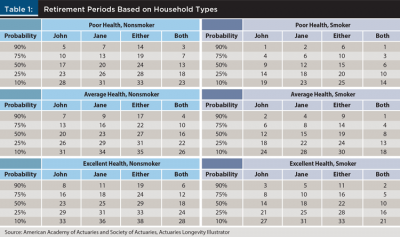
The median (50 percent) survival probability period, as well as other probability estimates, change materially based on the assumed attributes. For example, if the household is assumed to be in poor health and the members smoke, the median survival probability periods are 9, 12, 15, and 6 years for John, Jane, either or both, respectively. In contrast, if the household is assumed to be in excellent health and members don’t smoke, the median survival probabilities are 23, 25, 29, and 18 years for John, Jane, either or both, respectively. There is a roughly 15-year differential in these different periods, which is relatively constant across survival probabilities.
Changing the assumed length of retirement by 15 years can materially affect required savings or recommended spending levels, and it speaks to the importance of ensuring that mortality estimates are personalized to the respective household.
Do Financial Planners Change Mortality Assumptions for Clients?
The analysis so far suggests that there are factors than can significantly affect mortality rates (for example, client health and smoker status). An important question, though, is to what extent financial planners consider personalized mortality factors when establishing the retirement end date in a financial plan. To determine this, data is obtained from a financial planning platform available in Canada.
Data was filtered so that only those from the same country (Canada) are included. To be included, the plan must provide information on gender; the annual retirement income goal must be at least $10,000 (in the local currency); the minimum retirement age must be 50; and the assumed length of retirement must be at least five years. Fields available include the client’s age, client’s assumed retirement start age, client’s assumed retirement end age, and retirement goal. Age and gender fields are also available for the spouse, if provided. A total of 31,211 plans met the required filters from an initial dataset of 65,535 plans, with a total of 48,923 retirement end age estimates (the number of retirement ages exceeds the number of plans because some plans were for two people). Financial plans occurred between 2009 and 2020.
Figure 2 includes the distribution of retirement end age assumptions in financial plans by gender. The vast majority (97.2 percent) of retirement end age assumptions were multiples of five, between the ages 75 and 105, which is why only these multiples are included in Figure 2.
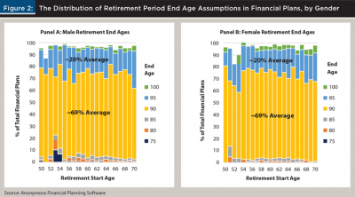
The distribution of retirement income ages is remarkably similar by gender and age, as well as by assumed retirement start age. Approximately 70 percent of retirement end ages were 90, whether male or female, and approximately 20 percent of retirement end ages were age 95. The average assumed retirement end age only increases by approximately two years for males, moving from a start age of 50 to 70 (89.8 to 91.9) versus 0.9 years for females (91.1 to 92.0).
Based on the 2013/2015 Canada Life Table, the life expectancy for a 65-year-old male was 19.1 years versus 22.0 for females. Therefore, a retirement end age of 90 would be approximately six years longer than life expectancy for a male and three years longer for a female. There is a 27.7 percent probability of a 65-year-old male surviving to age 90, versus a 40.1 percent probability for a female. Additionally, there is a 10.0 percent probability of a 65-year-old male surviving to age 95, versus a 19.0 percent probability for a female. Therefore, either retirement end age assumption (90 or 95) is clearly longer than life expectancy. The potential efficacy of these decisions will be discussed in a future section, especially as it relates to married couples.
An OLS regression was performed to better understand the variables related to retirement end age estimates. The dependent variable was the retirement end age, and independent variables included client age, client retirement age, client retirement goal, client gender, and whether the client was married. The results of the regression are included in Table 2.
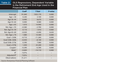
The regression results are interesting in a few respects. First, virtually all coefficients were significant at the 5 percent level. Second, it appears male life expectancy retirement end age values are only 0.6 years less than females, on average. The actual difference in life expectancies between males and females is closer to three years, and it doesn’t appear this difference is being accounted for. Third, life expectancy estimates are lower for those who are married. While the ultimate length of retirement is going to be based on whichever spouse is assumed to live longest, retiree households with two members face more tail risk, since the assets must fund a period so long as either is alive. Therefore, some additional margin should generally be assumed for a married couple versus a single retiree.
There is a notable effect by retirement income goal, where a client with an income goal exceeding $75,000 would have a retirement period that was roughly two years longer than someone with an income goal of $25,000, holding everything else constant. Additionally, retirement end ages appear to increase by age and when retirement is assumed to commence, consistent with how life expectancies evolve over a lifetime.
It is not clear how representative the information reviewed is of all financial plans (that is, it is not necessarily as representative of the decisions of financial planners like the Survey of Consumer Finances (SCF) and the Health and Retirement Study (HRS) are of U.S. households). However, the strong pull toward certain numbers (for example, age 90 and 95, as well as using ages that are a multiple of five) suggests that the majority of retirement end ages are likely not all that personalized to each client. Why financial advisers are not personalizing mortality estimates, and the approaches used to forecast end ages, definitely warrants additional research.
How to Model the End of Retirement in a Financial Plan
Households that use financial planners report higher average health, a lower probability of smoking, and higher income levels based on data in the 2016 SCF. Each of these attributes suggests that households that use financial planners are likely to have a longer retirement than the “average” American household. This is why Krueger (2011) suggests using the Society of Actuaries’ immediate annuity table, versus tables such as the Social Security Administration’s Period Life Table, when estimating survival probabilities in a financial plan. The 2012 Individual Annuity Mortality Table is the most recently released version (versus the 2000 version cited in the paper).
Even once suitable mortality rates have been determined, there is no consensus on the approach to estimate the length of retirement in a financial plan. In other words, planners using the exact same mortality table could reach very different conclusions about what a suitable length of retirement is for planning purposes. In this section, we explore how to determine a suitable value.
When determining the retirement period, it is important to consider the shortfall aversion metric used as part of the financial plan. Financial planners are increasingly relying on Monte Carlo projections, where the probability of success is the outcomes measure—that is, required savings or optimal spending are determined based on a target probability of success. While the probability of success is imperfect because it fails to capture the magnitude of failure, it allows for the introduction of uncertainty in financial plans and is therefore a more robust assessment of a given strategy than a pure deterministic forecast.
The only random variable in financial plans that incorporate Monte Carlo forecasts is typically returns (that is, returns are the only stochastic variable) and retirement is generally assumed to last a fixed period (for example, 30 years). In theory, mortality could be randomized as well, since first estimating a conservative retirement period (for example, one where there is only a 20 percent probability of outliving) and then overlaying a conservative shortfall target (for example, targeting a 90 percent success rate) can result in a level of required savings that is considerably higher than the true failure metric (that is, the probability of being broke while alive). Therefore, it’s important to consider the shortfall aversion metric when determining the retirement period to ensure the financial plan does not result in overly conservative estimates for required saving (or spending).
In theory, the length of retirement should be determined based on personalized mortality rates, and the target success rate (or shortfall aversion metric) should be related to the client’s risk aversion associated with accomplishing a goal. From this perspective, two clients with identical health situations retiring at the same age would have the same retirement period but could have very different target success rates based on their desired comfort around maintaining a certain standard of living during retirement. For example, the retirement period for both clients would be 30 years, but the client who is more risk-averse might have a target probability of success of 90 percent, versus 75 percent for the one who is more risk-tolerant.
Basing the retirement period on personalized mortality estimates and using the Monte Carlo simulation probability of success as the risk-aversion measure does not mean the retirement period should subsequently be based on life expectancy (that is, a roughly 50 percent survival probability). There are interaction effects at play when it comes to selecting the length of retirement, and it is assumed that length of retirement should generally be a period longer than life expectancy. This section explores how to estimate the appropriate period.
First, a series of Monte Carlo projections was performed. For the projections, the portfolio was assumed to be 40 percent equities and 60 percent fixed income, where the risk level remained constant through retirement. Equities had an assumed annual return of 8 percent and a standard deviation of 20 percent. Fixed income had an annual return of 4 percent and a standard deviation of 7 percent. The correlation between equity and fixed income was assumed to be 0.1, and there was an annual assumed 1 percent fee assessed to the portfolio. Inflation was assumed to be 2 percent. Returns were assumed to follow a normal distribution.
The households considered were male, female, and joint, where the joint household was composed of a male and a female the same age. All individuals were assumed to be age 65 and at retirement. Mortality rates were based on the Society of Actuaries Individual Annuity Mortality (2012 IAM) Table with improvement to the year 2020. Using these mortality rates, life expectancy, which equates to roughly a 50 percent survival probability, for a 65-year-old male was approximately 22 years, and 24 years for a 65-year-old female. The analysis considered 10,000 Monte Carlo runs.
The analysis estimated safe initial withdrawal rates, where the initial withdrawal amount was assumed to increase annually with inflation. This is consistent with the approach taken by Bengen (1994). While there is research that suggests retiree spending does not increase annually with inflation (for example, Blanchett 2014), assuming an annual increase with inflation is the most common assumption in financial plans today.
Table 3 includes the results of various projections. Panel A includes the initial safe withdrawal rates for various target probabilities of success and retirement periods. For example, if retirement were assumed to last 30 years and the target success rate were 90 percent, the initial portfolio withdrawal would be 3 percent. That initial withdrawal amount is then assumed to increase annually by inflation for the entire period.
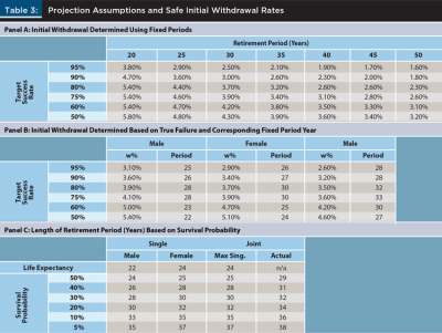
Panel B includes the initial safe withdrawal rates where “failure” is defined as the household being alive (either member if it is a joint household) and the portfolio not being able to sustain the withdrawal amount. In other words, the portfolio only fails if some member of the household is still alive when the assets have been depleted. This is obviously different from the traditional projection approach, which uses a fixed period, since this period considers mortality. The failure rates were determined by multiplying the respective success probabilities by the probability of the household dying in the respective year. To contrast Panel A with Panel B: Panel A determines failure rates over a fixed period of years, while Panel B determines failure based on whether any member of that household is still alive, based on the respective mortality rates. Panel C includes how long the assumed retirement period would last based on various target survival probabilities (that is, the probability of not outliving the retirement period), and includes life expectancies for John and Jane. The maximum joint period is the maximum value for either member of the respective couple, or the actual survival probability distribution for the couple.
Optimal initial withdrawal rates vary considerably based on the target retirement period and that target success rate (Panel A). Not surprisingly, optimal initial withdrawal rates that incorporate mortality rates also vary based on the assumed retiree household type (Panel B). Independently selecting a retirement period and a success rate can lead to a significantly different initial withdrawal rate than when they are considered jointly. For example, the 20 percent survival probability period for the couple is 34 years (Panel C). If a financial planner were to select the closest retirement period with a five-year increment (35 years), and select a relatively conservative success rate, such as 90 percent, the resulting initial withdrawal rate would be 2.6 percent. In reality, a 2.6 percent initial withdrawal rate has a 95 percent probability of success when incorporating mortality rates. In other words, a 2.6 percent initial withdrawal rate is actually safer than it appears when failure is defined through the lens of not having the desired income while alive versus a given fixed period. If the couple actually wanted to target a 90 percent success rate that incorporates mortality, their actual initial withdrawal rate should be 3.2 percent, which is 23.1 percent higher (3.2% / 2.6% = 1.231).
In theory, considering the distribution of survival rates of the household members is probably the best way to incorporate personalized mortality; however, these calculations can be complex, especially for a joint household (that is, estimating the probability of either member surviving to a given period). These survival rates are also not always available in online tools, which tend to focus on life expectancy. Therefore, a model is developed that keys off life expectancy and determines the additional number of years that should be added to life expectancy to result in a reasonable retirement period.
The analysis used the first implicate from each household from the 2016 Survey of Consumer Finances (SCF) to create a dataset of 6,248 potential retiree households. The assumed retirement need was based on the household type (joint or single) and assumed the retirement age for each individual was the age noted that funds would be withdrawn from retirement savings. If a value was not available, it was randomly seeded, assuming a mean of 65 with a standard deviation of three years. If it was a couple household, the spouse was assumed to retire at the same time, but there could be an age difference in spouses, which was assumed to be no greater than 20 years.
For each household, the probability of survival for each year was estimated using the mortality model introduced by Blanchett (2020).
For each household, the number of years that would need to be added to the life expectancy value to result in the actual target success rate (which considers mortality) was estimated. Median survival mortality was used for joint couples. Success rates of 95 percent, 90 percent, 80 percent, and 75 percent were targeted since they represent the general range of success rates used by planners.
The results are included in Table 4 for single households (Panel A), for joint households using the longer life expectancy of either couple (Panel B), and the median survival probability for the joint couple (Panel C). The probability of success reflects the actual assumed success rate targeted in the analysis, while the percentiles provide context on the distribution of respective solved periods.
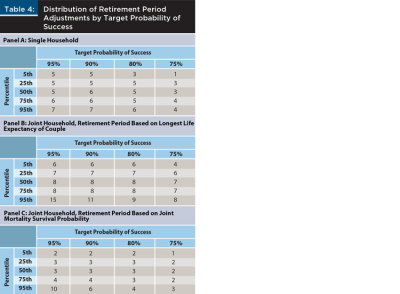
The results in Table 4 suggest that for a single household, adding five years to a personalized life expectancy estimate would be a way to estimate an appropriate retirement period (Panel A). For joint households, eight years should be added to the longest life expectancy of the two members (Panel B) to achieve a 95 percent chance of portfolio sustainability given a 75th percentile life expectancy, or three years if the retirement period considers the actual joint survival probabilities (Panel C).
The difference in the estimated add-on for joint households (Panel B) compared with single households (Panel A), which is approximately eight years versus five years, respectively, reflects the tail risks associated with joint households. Again, this suggests retirement end age estimates need to be longer for joint households. This is the opposite of the effect noted in financial plans reviewed, where end age estimates were lower for couples versus single households (see the regression results in Table 2).
The life expectancy for a 65-year-old female based on the Social Security Administration 2016 Period Life Table is 20.5 years, versus 23.9 years for the Society of Actuaries Individual Annuity Mortality (2012 IAM) Table with improvement to the year 2020. This suggests 30 years is likely a reasonable approximate assumed retirement period for the average 65-year-old couple (male and female) today, using the previously noted eight-plus years approach to estimating the retirement period. However, the optimal period will obviously vary significantly based on the attributes of the respective household.
Conclusions
The length of retirement is one of the most important assumptions in a financial plan. A variety of attributes can significantly impact the assumed length of retirement, such as health status, income, and whether the individual smokes, among other attributes. A review of financial planning assumptions in a financial planning program, though, suggests that retirement age assumptions are likely not that personalized in financial plans given the significant use of certain retirement end ages (for example, 90 and 95) and the focus on numbers with a multiple of five. Additionally, while the assumptions used appear reasonable for a single retiree, care should be taken when considering the length of retirement for a couple, given the tail risk associated with either member surviving significantly longer than average.
A model is introduced in this paper to determine a suitable retirement period. Through simulations, it is determined that adding five years to projected life expectancy for a single household and eight years to the longest life expectancy of either member of a joint household (or to each member if separate end ages are used), at retirement, is an appropriate retirement end age assumption if the outcome variable is the probability of success (using a Monte Carlo model) and only fixed periods can be modeled (mortality rates are not directly incorporated). This approach suggests a retirement period of 30 years (to age 95) is a reasonable assumption for the average 65-year-old male/female couple retiring today.
Similar to return estimates and other key assumptions in a financial plan, the retirement end age assumptions should be regularly reviewed to ensure they are timely and reflect all available information about both the client and mortality tables.
Endnotes
- See American Academy of Actuaries and Society of Actuaries, Actuaries Longevity Illustrator, www.longevityillustrator.org/ (accessed April 16, 2020).
- See www150.statcan.gc.ca/n1/pub/84-537-x/2019002/xls/2013-2015_Tbl-eng.xlsx. This represents the average of the respective financial plan date.
- See U.S. Federal Reserve’s “2016 Survey of Consumer Finances,” https://www.federalreserve.gov/econres/scf_2016.htm.
- See www.naic.org/store/free/MDL-821.pdf.
- The SCF imputes missing values using a multiple imputation method, where multiple values/responses are provided to represent the range of potential actual values. Each respondent has five sets of data (implicates), and the first of those five is used for the analysis.
References
Bengen, William. 1994. “Determining Withdrawal Rates Using Historical Data.” Journal of Financial Planning 7 (4): 171–180.
Blanchett, David. 2014. “Exploring the Retirement Consumption Puzzle.” Journal of Financial Planning 27 (5): 34.
Blanchett, David. 2020. “The Accuracy of Subjective Mortality Estimates.” Working Paper.
Blanchett, David and Brian Blanchett. 2008. “Joint Life Expectancy and the Retirement Distribution Period.” Journal of Financial Planning 21 (12): 54–60.
Krueger, Cheryl. 2011. “Mortality Assumptions:
Are Planners Getting it Right?” Journal of Financial Planning 23 (12): 36–37.
Citation
Blanchett, David M. 2021. “How to Estimate ‘The End’ of Retirement.” Journal of Financial Planning 34 (8): 88–99.