Journal of Financial Planning: August 2019
Javier Estrada, Ph.D., is a professor of finance at IESE Business School in Barcelona, Spain. He is also a partner and adviser at Sports Global Consulting Investments, a company that provides wealth management advice to professional athletes and other clients; and he is the sole adviser of the investment strategy of the Alpha Investments mutual fund.
JOIN THE DISCUSSION: Discuss this article with fellow FPA Members through FPA's Knowledge Circles.
Executive Summary
- Retirement accumulation plans are commonly based on expected returns, which are unlikely to be the same as those experienced by investors. Hence the question: when markets behave differently from what was expected, should individuals stick to their plan or adjust it?
- This paper evaluated dynamic strategies designed to keep the portfolio close to the path outlined in the financial plan, referred to as managing to target, or M2T.
- A static strategy of sticking to the plan was compared to dynamic strategies, and results showed that some of the M2T policies considered outperformed a static policy.
- Results also showed that adjusting periodic contributions was superior to adjusting the portfolio’s asset allocation.
Do your clients have a target balance for their portfolio on their retirement date? Do they have a plan to hit that target, including the periodic contributions they should make to their retirement portfolio? Have they thought about the asset allocation they should have, and how it should evolve during the accumulation period? Should clients consider making contributions that depart from their financial plan and under what conditions? These are the critical questions discussed in this paper.
Casual evidence suggests that many individuals do not have a clear financial plan to build a retirement portfolio. Most people do not even have a target value for such a portfolio on the retirement date, a figure often referred to as “the number” (Eisenberg 2006). This may be because “the number” depends on both life expectancy and the cost of the desired lifestyle during retirement, neither of which individuals may find easy to forecast, particularly in the early stages of their working years.
This paper does not deal with how to determine a target amount for a retirement portfolio. Rather, it takes “the number” as given and: (1) outlines a financial plan to hit the target; (2) compares a static strategy of sticking to the plan to dynamic strategies that make adjustments to the plan along the way; and (3) proposes a way to evaluate investment strategies for the accumulation period in order to determine the best course of action.
The financial plan designed to hit a target retirement portfolio balance consists of determining the inflation-adjusted constant annual contribution during the expected number of working years, given a selected asset allocation. The individual can stick to the contributions and asset allocation specified in the plan (inevitably based on expected returns) and hope that the actual returns obtained during his working years will lead him to meet, or at least end up close to, his target amount.
Alternatively, if actual returns push the portfolio away from the path specified in the plan (referred to here as the expected path), the individual could adjust his annual contributions or the asset allocation to bring the portfolio back to the expected path. The question addressed in this paper is whether engaging in such dynamic adjustments is beneficial. Those adjustments are a set of policies broadly referred to here as managing to target (M2T).
Three types of M2T policies were considered. The first group were effective, but impractical, because they may require an individual to adjust their periodic contributions more than they may be able or willing to tolerate. The second group were feasible but limited; they were easier for an individual to tolerate but generally yielded lower benefits than the first group. The third group were asset allocation policies that stuck to the contributions specified in the financial plan but adjusted the asset allocation over time.
To determine whether to implement the contributions and asset allocation outlined in the plan, or to make dynamic adjustments along the way, the individual needs a criterion to decide. One way to make this decision is to compare the size of the portfolio on the retirement date across the strategies considered. However, this is appropriate only if the periodic contributions of the different strategies are the same; if they are not, then an alternative criterion is needed. The tool proposed here to evaluate investment strategies during the accumulation period is a strategy’s net present value.
The results of this analysis showed that: (1) some dynamic policies outperformed a static policy of simply sticking to the plan; (2) adjusting the periodic contributions had a larger impact than adjusting the portfolio’s asset allocation; and (3) there was a trade-off between tolerating flexibility in the contributions and the benefits obtained from dynamic adjustments.
Literature Review
The debate between static and dynamic strategies (both accumulation and withdrawal) has a history in the financial planning literature. Although not strictly related to the issues discussed in this analysis, Bengen’s (1994) pioneering article introducing the 4 percent rule prompted additional research and analysis between fixed and variable withdrawal rates. Over 20 years later, broad consensus has not been reached.
More closely related to the issues discussed in this analysis, another debated topic focuses on whether to implement a static or dynamic asset allocation. This issue has been explored both for the accumulation period and for the retirement period. Regarding the latter, Pfau and Kitces (2014) advocated for a dynamic asset allocation with a rising equity glide path—a strategy that makes the portfolio more aggressive as the retiree ages. Conversely, Estrada (2016) found support for a declining equity glidepath, making the portfolio increasingly more conservative. Blanchett (2007); Kitces and Pfau (2015), and Estrada (2016) advocated for aggressive static asset allocations that maintained a high proportion of stocks, and each highlighted the effectiveness of the 60/40 stock-bond (static) allocation.
Regarding the accumulation period, which is the focus of this analysis, the conventional wisdom favors a dynamic strategy with a declining equity glide path (a portfolio that becomes gradually more conservative as the retirement date approaches), such as those implemented by target-date funds. However, there is little consensus in the research on the superiority of this approach.
Basu and Drew (2009); Arnott, Sherrerd, and Wu (2013); and Estrada (2014) all found that rising equity glide paths outperformed declining equity glide paths as far as capital accumulation was concerned. Put differently, if individuals aim to maximize the size of their nest egg on the retirement date, they should make their portfolios more aggressive over time. That said, Dolvin, Templeton, and Rieber (2010) advocated for a very aggressive static allocation until some 10 years before retirement, after which the portfolio should become gradually more conservative. Estrada (2014) also found support for a very aggressive static allocation, but throughout the accumulation period.
Much of the prior research on accumulation strategies has failed to incorporate a target portfolio on the retirement date, as was done here. An exception is Basu, Byrne, and Drew (2011), which incorporated an accumulation target that, together with portfolio performance, determined whether to periodically switch from stocks to bonds or vice versa. Most of the research on the accumulation period has focused on adjustments to the portfolio’s asset allocation, and has largely ignored adjustments to the periodic contributions, as was done here.
Assumptions and Calculations
Financial plan assumptions. Consider a 25-year-old individual who plans to work for 40 years and aims to retire with a $1 million portfolio in real (inflation-adjusted) dollars (determining the appropriate size of the portfolio is far from trivial; however, within the scope of this analysis, “the number” is taken as given).
This individual plans to make annual contributions to his retirement portfolio, constant in real terms, starting at the end of his first working year and ending one year before retirement (that is, on his retirement date he does not make a contribution but rather liquidates the portfolio), for a total of 39 annual contributions.
The portfolio consists of 60 percent stocks and 40 percent bonds. Over the 1900 to 2017 period, an annually rebalanced, 60/40 portfolio of U.S. stocks and bonds delivered an annualized real return of 5 percent. Consider, then, that figure as the expected annual return of our individual’s portfolio.
Find the constant annual real contribution (C), given the number of contributions to be made (T), the portfolio’s expected annual real return (R), and the target retirement portfolio (P*) that solves the expression:
Note that P0 = C40 = 0 and Ct = C for t = 1, …, 39; that is, the portfolio starts with 0, the next 39 contributions are constant, and there is no contribution at the end of the working period when the portfolio is simply liquidated.
In our specific example, the individual needs to solve the expression:
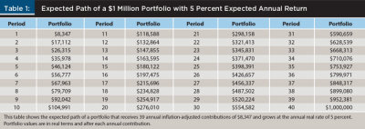
In other words, if our individual makes annual (inflation-adjusted) contributions of $8,347 during the 39 years, and his portfolio grows at the annual real rate of 5 percent, then he will retire after 40 years with the target $1 million portfolio.
Putting together the constant annual real contributions ($8,347) and the expected return of the portfolio (5 percent) yields the portfolio’s expected path, shown in Table 1. This expected path plays the critical role of being the benchmark against which deviations from the plan are measured; in other words, dynamic adjustments are considered only when the actual portfolio deviates from this expected path.
Keep in mind that although it is called an “expected” path, in any given accumulation period, our individual’s 39 annual contributions of $8,347 to a 60/40 stock/bond portfolio are likely to result in a nest egg higher or lower than the $1 million target.
Evaluating strategies. The standard way to evaluate an investment strategy during the accumulation period is to assess its terminal value (the value of the portfolio on the retirement date) over a large number of historical or simulated accumulation periods. This amounts to comparing several parameters or percentiles of the distribution of terminal values (Basu, Byrne, and Drew 2011; Arnott, Sherrerd, and Wu 2013; and Estrada 2014).
That approach is plausible as long as the periodic contributions of the strategies considered are the same. However, over time an individual may adjust their periodic contributions, in which case focusing just on terminal values would be misleading. Given the stream of negative cash flows (contributions) and the final positive cash flow (the retirement portfolio), a tool typically used to evaluate investment projects, the net present value (NPV), appears useful as a metric to evaluate accumulation strategies. For this reason, the strategies considered in the analysis were evaluated with the expression:
where Ct is a strategy’s contribution in year t; R is the strategy’s required return; and P40 is the value of the portfolio on the retirement date.
Another possibility for the evaluating accumulation strategies is to consider a strategy’s internal rate of return (IRR). If the cash flows change in sign just once (from inflows to outflows or vice versa), then both the NPV and IRR approaches would provide the same assessment (as would be the case when all the contributions are negative cash flows and the liquidated portfolio is a positive cash flow). However, it is possible to conceive strategies where if the individual is above his expected path, he could make a withdrawal from the portfolio (rather than a contribution), thus generating a positive cash flow. And when cash flows change signs more than once, a unique solution for the IRR is not guaranteed. For this reason, comparing NPVs provides a slightly more general way of assessing accumulation strategies than comparing IRRs.
The sample consisted of annual stock and bond returns for the U.S. market between 1900 and 2017. Stocks were represented by the S&P 500 and bonds by 10-year Treasury Notes, both in their total return version (including capital gains/losses and cash flows paid), downloaded from Global Financial Data (globalfinancialdata.com). All returns were real, adjusted by inflation as measured by the Consumer Price Index. During the 118-year period considered, stocks and bonds delivered annual returns of 6.4 percent and 1.6 percent, respectively, with annual volatility of 20 percent and 9.4 percent, respectively. Their correlation over the sample period was 0.23.
All strategies considered were evaluated over all the possible historical 40-year periods between 1899 and 2017; this yielded 80 accumulation periods, beginning with 1899 to 1938 and ending with 1978 to 2017.2 Each strategy was therefore exposed to 39 years of returns over each of the 80 accumulation periods considered, resulting in 80 NPVs per strategy, which in turn resulted in a distribution of NPVs for each strategy. These distributions are the basis of the evaluation of the different strategies considered below.
Accumulation Strategies
The first policy considered was the stick to the plan (S2P) strategy, in which 39 annual real contributions of $8,347 were made, regardless of whether the portfolio was on track toward the $1 million target. This strategy was the benchmark against which the dynamic policies were evaluated.
Three types of dynamic policies were considered—all with the goal of returning the portfolio (at least close) to the expected path outlined in the financial plan. These strategies are broadly referred to as managing to target (M2T).
Some M2T policies may be effective but impractical because they require the individual to do something he may be unable or unwilling to implement. Consider, for example, a strategy that in some years requires contributions many times larger, in real terms, than that made at the beginning of the accumulation period; or another whose contributions vary widely from year to year. Five such effective but impractical (EBI) policies were considered.
The first of these strategies (EBI1) made a positive or negative contribution (i.e., a withdrawal from the portfolio), so that at the end of each year the portfolio returned to the expected path outlined in Table 1. For example, if at the end of the second working year the portfolio had $12,112, the individual would contribute $5,000 so that the portfolio was left with the $17,112 balance outlined in the expected path. This strategy may result in very variable annual contributions (as will be seen below) even under normal market conditions. Furthermore, it is the only of all the strategies considered in this analysis that allowed for withdrawals from the portfolio.
The second of these strategies (EBI2) limited the annual contributions to no more than 5 percent above or below the contribution made the previous year. It aimed to limit the variability in contributions resulting from EBI1 and to avoid withdrawals from the retirement portfolio. The other three EBI strategies considered were similar but limited the annual contributions to no more than 10 percent (EBI3); 15 percent (EBI4); and 20 percent (EBI5) above or below the contribution made the previous year. In all cases, contributions were increased (decreased) when the portfolio was below (above) the value outlined in the expected path.
The next set of M2T policies evaluated had pros and cons relative to the EBI strategies. The main benefit was that they limited, in a greater way, the variability of the annual contributions, thus making them more realistic; the associated cost is that they also limited the benefits they produced. Five such feasible, but limited, (FBL) strategies were considered, limiting the annual contributions to no more than 5 percent (FBL1); 10 percent (FBL2); 15 percent (FBL3); 20 percent (FBL4); and 50 percent (FBL5) above or below the contribution made at the beginning of the accumulation period ($8,347). Once again, in all cases, contributions were increased (decreased) when the portfolio was below (above) the value outlined in the expected path.
The final set of M2T polices did not adjust the annual contributions. Rather, every five years the portfolio’s asset allocation was adjusted so that it became more aggressive (conservative) when the portfolio was below (above) the value outlined in the expected path.3 Three such asset allocation (AA) strategies were considered; the first limited the change in the asset allocation to 10 percentage points (AA1); the second to 20 percentage points (AA2); and the third to 30 percentage points (AA3).
Results
Table 2 summarizes the performance of the stick-to-the plan and effective, but impractical, strategies. Panel A of Table 2 summarizes the median of the distribution of NPVs, as well as its 5 percent (P5) and 10 percent (P10) cutoff points in the lower tail. Panel B focuses on the distribution of the value of the portfolio on the retirement date and reports its median, as well as the proportion of times it fell short of $1 million by 5 percent or more (Short5) and by 10 percent or more (Short10). Panel C reports the minimum and maximum annual contributions of the 3,120 contributions (39×80) made by each strategy.
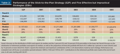
The S2P strategy was the benchmark against which all the M2T strategies were evaluated, and a strategy’s NPV was the metric used for the evaluation. Therefore, the median NPV of $15,259, as well as the 5 percent and 10 percent cutoff points in the lower tail of the distribution (–$52,697 and –$46,999) shown in panel A of Table 2 are important reference points. So are the median value of the portfolio on the retirement date ($1,107,423), and the proportion of times the portfolio was 5 percent and 10 percent short of $1 million on that date (29 percent and 24 percent of the periods considered), as shown in panel B of Table 2.
The question posed in this analysis is whether the representative subject could do better than simply sticking to his plan. Is there any value in implementing dynamic adjustments during the accumulation period so that the portfolio remains close to the expected path? The last five columns of Table 2 aim to answer this question for the five EBI strategies considered.
Panel A of Table 2 shows that all the EBI strategies outperformed the S2P strategy; they all have higher median NPV, as well as higher 5 percent and 10 percent cutoff points in the lower tail. The EBI strategies added value by increasing both average performance and performance in “bad scenarios” (defined as those in the lower 5 percent and 10 percent of the distribution). Based on these variables, EBI5 delivered the best performance.
Panel B of Table 2, which focuses on the value of portfolios on the retirement date, shows results broadly consistent (albeit more mixed) with those of panel A. Note that with the exception of EBI1, all other EBI strategies delivered a higher median value of the retirement portfolio. That said, it is important to highlight that the goal of the M2T strategies considered here was not to enhance the value of the retirement portfolio; rather, it was to hit (or end up close to) the $1 million target.
Of course, if the target is going to be missed, it is better to end up with more rather than with less than $1 million, which is the focus of the next two rows of panel B. These figures show that all EBI strategies mitigated the proportion of shortfalls relative to those of the S2P strategy, and that they did so in different degrees. From this perspective of limiting shortfalls, EBI3 seems to have delivered the best overall performance.
Finally, panel C shows why the EBI strategies were impractical. Using the initial annual contribution of $8,347 as a reference point, note that all strategies made contributions much higher than this amount, in real terms. In the case of EBI3, for example, the $39,325 contribution was almost five times larger than the initial contribution, something that many individuals may be unable or unwilling to implement. EBI1, on the other hand, revealed itself as the most impractical of all the EBI strategies, given that in one period, the representative individual could have withdrawn $249,660 from his portfolio, and in another he would have had to contribute $266,393.4
The empirical impracticality of EBI policies opens the door to explore the feasible, but limited, (FBL) policies outlined earlier. Table 3 summarizes their performance. Panel A of Table 3 shows that all FBL strategies outperformed the S2P strategy both in terms of average performance (an increase in the median NPV between 9 percent for FBL1 and 69 percent for FBL5) and performance in “bad” scenarios (an increase in its 5 percent cutoff points in the lower tail between 3 percent for FBL1 and 21 percent for FBL5, and an increase in its 10 percent cutoff points between 3 percent for FBL1 and 25 percent for FBL5). Note that the more flexibility in the contributions FBL strategies allowed for, the higher the benefits they provided.
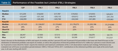
Panel B of Table 3 reinforces the results of panel A. Not only did all FBL strategies outperform the S2P strategy but also, as shown in panel A, the outperformance increased in the flexibility tolerated in the contributions. This is reflected by the fact that the average size of the retirement portfolio monotonically increased, and the proportion of shortfalls monotonically decreased from FBL1 to FBL5.
Panel C of Table 3 again provides a reality check by highlighting the trade-offs involved. FBL5 delivered the best overall results, but it forced the individual to contribute more than he may be willing or able to do, as reflected in a contribution 50 percent higher, in real terms, than that made at the beginning of the accumulation period. The individual may choose to limit the increases in annual contributions (move to the left in the table), but that would also limit the benefits he would obtain from trying to remain close to the expected path.
Comparing Table 2 and Table 3 further highlights the relevant trade-offs. FBL policies had the advantage of more predictable, and largely feasible, contributions; each FBL strategy limited the annual contributions to just three possible values ($8,347, x percent above, and x percent below), whereas EBI strategies displayed much more variable and extreme contributions. On the other hand, in terms of NPV (on average and in bad scenarios) and the final value of the retirement portfolio (on average and in terms of shortfalls), FBL strategies generally underperformed EBI strategies.
The final set of M2T policies evaluated did not adjust the contributions, but rather the portfolio’s asset allocation. Table 4 summarizes the performance of the three asset allocation (AA) policies outlined earlier, reporting the S2P strategy performance for reference. Panel A of Table 4 shows that these policies substantially underperformed the S2P strategy—both in terms of median NPV and NPV in bad scenarios.5
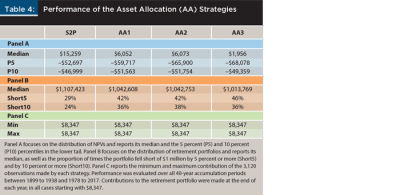
Panel B of Table 4 reinforces the previous results by showing that AA policies underperformed the S2P strategy in terms of the value of the retirement portfolio, both on average and in terms of shortfalls. More aggressive adjustments to the asset allocation (moving to the right in the table) did not lead to better results; in fact, as shown in panels A and B, the opposite seemed to be the case. Panel C simply shows that the annual contributions were not the variable used in these strategies to attempt to return the portfolio close to the expected path.
Tables 2, 3, and 4 reveal that, in terms of NPV (both on average and in bad scenarios) and in terms of the retirement portfolio (both on average and in terms of shortfalls), AA policies underperformed all the EBI and FBL strategies considered. If the goal is to keep a portfolio on track along its expected path, adjusting contributions was shown here to be more effective than adjusting the asset allocation.
The fact that AA strategies underperformed EBI and FBL strategies, and to a large degree, is perhaps not surprising. The latter policies adjusted annual contributions, and its impact on the portfolio was immediate and in a positive direction. The former policies, on the other hand, adjusted the asset allocation, but nothing guarantees that a more aggressive or conservative portfolio will perform as expected in the short term. In other words, AA policies took longer to impact the portfolio and may have initially done so in a negative direction.
Caveats and Future Research
A strategy that may sound plausible in a superficial analysis (such as having a financial plan and sticking to it—the EBI1 strategy in this analysis), has bad results in practice. Not only did EBI1 imply a volatility in contributions that no investor would likely be willing or able to bear, it also underperformed most of the other strategies considered.
Somewhat related, individuals and planners may not welcome the volatility in contributions that some of the strategies analyzed here implied. Although this may seem to limit the applicability of these strategies, note two things: (1) planners may offer a trade-off to clients— be willing to adjust your contributions and improve your results, or just stick to the plan outlined and obtain inferior results; and (2) the evidence discussed shows that even a little bit of flexibility (adjusting contributions by 5 percent up or down with respect to the initial contribution) led to improved results.
Throughout this analysis, the benchmark asset allocation used was 60 percent in stocks and 40 percent in bonds, and it was assumed to be constant during the accumulation period (except in the asset allocation policies). The allocation’s static nature may be questionable, particularly given the standard policy followed by target-date funds to make the asset allocation more conservative over time. The framework presented in this paper could accommodate a dynamic allocation in the financial plan.
Some individuals may want to do better than their stated target. Doing better has a cost counterpart: the individual would need to make higher contributions. This trade-off is captured in the NPV calculation. The results showed that the median nest egg of FBL strategies was 10 percent to 20 percent higher than the $1 million target.
Conclusion
When setting a target for a retirement portfolio and determining the periodic contributions that are expected to lead to it, the individual is essentially specifying a financial plan summarized by the expected path of his portfolio. A possible accumulation strategy is simply to stick to the contributions outlined in the plan and hope to hit (or end up close to) the number chosen. An alternative strategy is to take a more dynamic approach and introduce adjustments—either to periodic contributions or to the asset allocation— when the portfolio deviates from its expected path.
The evidence discussed, based on long-term data for the U.S. market, suggests that adjusting the periodic contributions was far superior to adjusting the asset allocation. Furthermore, of the feasible adjustments to the contributions discussed (the FBL policies), results showed that the more flexibility an individual was able or willing to accept in the periodic contributions, the larger are the benefits obtained.
The benefits obtained from these dynamic policies, relative to a static strategy, were twofold: (1) improved average performance and performance in bad scenarios as measured by their NPV; and (2) larger nest eggs on the retirement date and reduced proportion of shortfalls from the target portfolio chosen.
The results discussed here suggest that it is critical for individuals to have a financial plan, to periodically assess whether their plan is on track, and if it is not, to introduce adjustments to the periodic contributions to their retirement portfolios.
Endnotes
-
None of these assumptions are critical. The size of the target retirement portfolio and the number of years working and making contributions do not affect the key messages that stem from the analysis. The analysis performed would easily accommodate any plan for the contributions made during the accumulation period. The only restriction is that there has to be a plan; without it, the expected path cannot be calculated and there would be no benchmark to assess deviations from the plan.
-
The analysis started with 1899 because the stock and bond returns in the sample started in 1900. Because the representative individual made his first contribution at the end of the first working year, he started his 60/40 stock/bond portfolio with $8,347 at the beginning of 1900 and was therefore exposed to the returns of these two asset classes during the first year of returns available from the sample.
-
If the three AA strategies considered adjusted the asset allocation annually instead of every five years, their results (not reported) would be worse than those displayed in Table 4. Unreported results also show worse results if the asset allocation were to be adjusted every 10 years instead of every five years.
-
Adding to the implausible results of the EBI1 strategy is the fact that withdrawals are highly penalized in 401(k) plans. Still, it is interesting to see that having a plan and sticking to it may seem to be a good idea until the implications and results of the strategy are evaluated. What seems to be a plausible strategy in an analysis can turn out to be a bad strategy from a practical point of view.
-
Note that the distributions of NPVs of the asset allocation policies were much more positively skewed than all the other NPV distributions considered. To illustrate, the mean and median NPV for the S2P policy were $20,445 and $15,259, respectively, whereas those of the AA1 policy were $18,731 and $6,052, respectively.
References
Arnott, Robert, Katrina Sherrerd, and Lillian Wu. 2013. “The Glidepath Illusion … and Potential Solutions.” Journal of Retirement 1 (2): 13–28.
Basu, Anup K., and Michael E. Drew. 2009. “Portfolio Size Effect in Retirement Accounts: What Does It Imply for Lifecycle Asset Allocation Funds?” Journal of Portfolio Management 35 (3): 61–72.
Basu, Anup, Alistair Byrne, and Michael Drew. 2011. “Dynamic Lifecycle Strategies for Target Date Retirement Funds.” Journal of Portfolio Management 37 (2): 83–96.
Bengen, William. 1994. “Determining Withdrawal Rates Using Historical Data.” Journal of Financial Planning 7 (4): 171–180.
Blanchett, David. 2007. “Dynamic Allocation Strategies for Distribution Portfolios: Determining the Optimal Distribution Glide Path.” Journal of Financial Planning 20 (12): 68–81.
Dolvin, Steven, William Templeton, and William Rieber. 2010. “Asset Allocation for Retirement: Simple Heuristics and Target-Date Funds.” Journal of Financial Planning 23 (3): 60–71.
Eisenberg, Lee. 2006. The Number: What Do You Need for the Rest of Your Life, and What Will It Cost? New York, N.Y.: Simon & Schuster.
Estrada, Javier. 2014. “The Glidepath Illusion: An International Perspective.” Journal of Portfolio Management 40 (4): 52–64.
Estrada, Javier. 2016. “The Retirement Glidepath: An International Perspective.” Journal of Investing 25 (2): 28–54.
Kitces, Michael, and Wade Pfau. 2015. “Retirement Risk, Rising Equity Glide Paths, and Valuation-Based Asset Allocation.” Journal of Financial Planning 28 (3): 38–48.
Pfau, Wade, and Michael Kitces. 2014. “Reducing Retirement Risk with a Rising Equity Glide Path.” Journal of Financial Planning 27 (1): 38–48.
Citation
Estrada, Javier. 2019. “Managing to Target: Dynamic Adjustments for Accumulation Strategies.” Journal of Financial Planning 32
(8): 46–53.