Portfolio Optimization Theory Versus Practice

Journal of Financial Planning: April 2013

Executive Summary

• This paper examines the gap between the theory of portfolio construction and its practice. In particular, it analyzes some of the problems in the application of portfolio optimization techniques to individual investors. We then discuss what can be done today to compensate for the problems with the theory, and what additional work needs to be accomplished.
• Various books and articles have discussed some of the problems with modern portfolio theory, which is the basis for most portfolio optimizers. This article compiles that information into a critique of the investment industry’s continued reliance on portfolio optimization tools.
• Clients and investment professionals alike place far too much faith in the mathematics of portfolio optimization techniques and the recommendations that result from applying optimization techniques to clients’ portfolios. Clients will benefit from being more aware of the very substantial gap between asset allocation theory and the real world. Portfolio construction is mostly an art, not a science. Investment success depends upon experience, judgment, skill, and luck—the latter often showing up as fortuitous timing. Clients should avoid relying too much upon the seemingly precise construction of “optimum” portfolios and risk measurements produced by portfolio optimization tools.

Roy Ballentine, CFP^®, CLU^®, ChFC^®, is the chairman of the board, CEO, and founder of Ballentine Partners LLC, based in Wolfeboro, New Hampshire.

Nearly all investment professionals rely upon portfolio optimization techniques grounded in modern portfolio theory, (MPT) to structure investment portfolios for individual investors. Using statistical techniques and computer-assisted modeling, investment advisers are able to combine different types of assets, such as stocks, bonds, cash, real estate, and hedge funds, to create portfolios that claim to offer the best possible return for specified levels of risk, or to minimize the amount of risk an investor must assume to achieve a specified amount of return.

The problem is that the real world does not always fit the theory perfectly. Sometimes, reality and theory are not even close. The famous phrase often attributed to Yogi Berra, “In theory there is no difference between theory and practice. In practice there is,”¹ certainly applies to portfolio optimization techniques as practiced today. The remainder of this paper presents theoretical assumptions and generalities found in MPT with commentary from a “practice” perspective.

Problems with Portfolio Optimization Models

We begin with an analysis of the assumptions underlying most portfolio optimization models. Following is a comparison of the gap between theory and practice.

Theory: The composition of each asset class is well defined and stable.

Practice: Asset classes are not well defined, and they are not stable.

Within the investment management field, there is no universally accepted definition of “asset class.” Private investors (and many investment professionals) who rely upon portfolio optimization models for assistance in portfolio construction typically ask very few questions about how asset classes are defined, how the composition of an asset class may have changed over time, and whether the historical data often used to estimate the future behavior of an asset class is appropriate for that purpose.

What actually distinguishes an asset class? How many asset classes are required to describe the universe of equities—just one or several? Are hedge funds an asset class, or should they be considered a subset of global equities? There are no clear answers to these questions.

The composition of any asset class is not likely to remain stable for very long. For example, in the portfolio optimization process, the equities of emerging markets are often represented by one of the emerging market indices. The composition of those indices has changed substantially over time. China and India are now among the world’s largest economies, but they are still included in the emerging market indices. Is it reasonable to estimate the future behavior of China’s economy based on the past results for an emerging market index? Sometime soon China will no longer be indexed as an emerging market. The same sorts of questions could be asked about almost any asset class.

Theory: Each asset class can be represented by an index or some other metric that represents the
performance of the asset class.

Practice: Although it is commonly thought that there are universally accepted benchmarks for any asset class, the reality is that no general consensus exists and any number of benchmarks can be found. With some asset classes, investors face significant challenges to find data to support estimates of return, risk, and correlation. Unfortunately, some of the asset classes that seem to provide the most diversification benefits for investors are the asset classes for which investors have the least reliable performance data.

For example, when private equity first captured the attention of individual investors, there were only a handful of private equity funds. Investors were attracted to the high returns and diversification benefits that private equity seemed to offer. Now there are many private equity firms and competition is fierce. Private equity benchmarks that rely upon historical returns for private equity may not be a fair representation of today’s highly competitive private equity market. Venture capital, hedge funds, real estate, and commodities² suffer from similar performance measurement problems, which present a very serious challenge in the portfolio construction process.

Theory: The only factors that matter in portfolio construction are the final portfolio’s expected return and its risk parameters.

Practice: Investors certainly care about a portfolio’s expected return and the relationship between risk and return, but they also care about an array of other factors—none of which are taken into account by most portfolio optimization models, such as the following. This is where the financial planner can prove his or her value:

• How much annual cash flow does the investor require from the portfolio?
• How much income tax will the investor have to pay on investment income?
• How liquid is the portfolio, in case the investor needs access to immediate cash?
• What is the unit purchase size for each asset class? The unit purchase size requirements for top-notch hedge funds, venture capital, private equity, and private real estate funds may be beyond the reach of many private investors, including investors who are considered to be very wealthy.
• What are the diversification requirements for each asset class? For example, various studies have found that an investment in at least eight funds with different strategies is required to achieve strategy diversification (Lhabitant and Learned 2002). Diversification requirements for private equity, venture capital, and private real estate may require making new investments over a period of many years to achieve time diversification. In addition to strategy diversification, manager diversification must be considered.
• How much manager selection risk³ is associated with a particular asset class recommendation? Is the investor able to tolerate the consequences of a manager selection mistake?
• Over what time frame is the investor planning to measure the portfolio results? Obviously, an investor who expects to live only a few years more and whose estate needs cash to pay estate taxes has a very different time frame than an investor who needs retirement income for 30 years or more.
• What are the consequences for the investor if the portfolio fails to perform as well as expected? An investor who needs funds on a specific date to pay a liability as it comes due faces different consequences than a wealthy grandparent who is investing to provide grandchildren with tuition assistance.

Theory: Investors are able to develop a sufficiently accurate forecast for each asset class that describes the mean return, standard deviation of returns, and the correlation of returns between all relevant asset classes for any given time period.

Practice: It is highly doubtful that anyone can consistently and accurately forecast the previous factors. Most forecasts rely heavily upon historical return data. If investment returns in each asset class have a tendency to revert to the mean, then a forecast based on historical data will tend to show a perverse bias favoring asset classes that may under-perform in the future.

The portfolio optimization process requires the following data elements as inputs for each asset class being considered for inclusion in the portfolio: average expected return, standard deviation of returns, and correlation of returns with every other asset class being considered.

How many input variables is that? Assume that 10 asset classes are being considered. A portfolio optimization model requires 10 estimates for average returns, 10 estimates for standard deviations of returns, and 45 correlation factors. That’s a total of 65 variables that must be correctly forecast.⁴

What is the likelihood someone will be able to forecast returns, standard deviations, and correlations for multiple asset classes for a multi-year period with sufficient accuracy to produce a portfolio recommendation that is optimal, or nearly optimal? How much does it matter if the various elements of the forecast are inaccurate? It matters a lot, particularly with respect to the expected return for an asset class. A relatively small change in the expected return can cause the recommended investment portfolio to change substantially.

Theory: A rational investor would want to own a portfolio that lies on the (unconstrained) efficient frontier, because those portfolios will produce the highest return for any given level of risk. That is, the portfolios on the efficient frontier are the most desirable portfolios.

Practice: It is highly unlikely any rational individual investor would want to own a portfolio that lies on the efficient frontier.

Financial planning practitioners familiar with portfolio optimization techniques know portfolio recommendations produced by an unconstrained optimization are likely to be dominated by a small set of asset classes that happen to have favorable forecasts at that moment. If the return estimates are based on historical data, the recommended portfolio may be concentrated in asset classes that have performed well recently. It is likely at least some of the recently hot asset classes are now over-valued and about to perform poorly.

Would a rational investor prefer a highly concentrated portfolio thought to lie on the efficient frontier over a more broadly diversified portfolio that lies some distance from the efficient frontier? Perhaps, but only if the investor has a high level of confidence in the forecast for each asset class. In the author’s experience, most investors have very little confidence in the forecast. Most advisers have so little confidence in their forecasts they are unwilling to recommend the portfolios produced by the unconstrained optimization process.

One solution to this problem is to constrain the inputs to the portfolio optimization process so as to force the optimizer to produce a broadly diversified portfolio. The constraints usually include both a maximum or minimum percentage of the portfolio’s capital allocated to each asset class. The constraints thus imposed change the location and the shape of the efficient frontier, so the recommended portfolio may then lie on the efficient frontier.

But, that is an admission the portfolio design process is mostly art wrapped in a veneer of scientific analysis. The adviser is forcing the optimization process to produce a preconceived result. In the author’s opinion, forcing the optimization process to produce a preconceived result is preferable to basing a recommendation on the unconstrained results of the optimization process. It is also an admission that, although the mathematics of portfolio optimization may be robust, the portfolio optimization process requires a liberal dose of experience and judgment.

Theory: The future pattern of returns for all asset classes can be accurately represented by a linear probability distribution, similar to the familiar bell curve.

Practice: The distributions of returns for most asset classes do not follow the familiar pattern of the bell curve, or normal distribution. In a normal distribution, the probability an investment return will fall far above or below the mean—that is, more than three standard deviations from the mean, is very low.

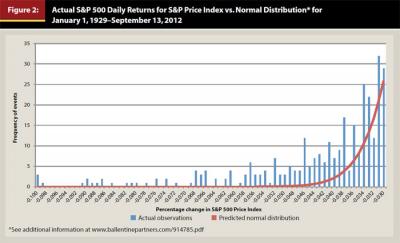
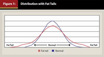
Actual investment returns are far more likely to fall more than three standard deviations above or below the mean than would be predicted if actual returns were normally distributed (Mandelbrot and Hudson 2004). The actual distribution of investment returns for most asset classes have “fat tails,” and are negatively skewed. The distribution of investment returns may follow some sort of exponential law, for which we currently do not have good modeling techniques. If the distribution of investment returns in the real world has fat tails and is negatively skewed, then the probability of extreme losses is much higher than is implied by standard risk models (see Figure 2).

The pioneers who developed MPT understood that investment returns cannot be adequately described by a normal distribution. Later, in the 1960s, Benoit Mandelbrot suggested investment returns are best described by a Stable Pareto distribution (Mandelbrot 1963). That type of distribution has fatter tails than a normal distribution, meaning that the probability of extreme events is higher. The distribution also can be skewed. Working with a Stable Pareto distribution requires highly specialized mathematical techniques. Interest in this problem died off until recently because the log-normal distributions commonly used for portfolio optimization seemed to do an adequate job. The stock market collapse of 2008 rattled the sense of complacency that built up around this problem.

Figure 1 compares a normal linear distribution to a distribution with fat tails (Rivera 2013). Although the differences between the two curves shown in Figure 1 may not look very significant, the amount of error introduced by assuming that investment returns can be described by a normal linear distribution is substantial. One consequence is the risk of loss in each asset class is significantly underestimated, and the risk of loss in the recommended portfolio may be considerably higher than is implied by the estimates produced by portfolio optimization models.

How far off are the risk estimates? According to risk estimates produced by portfolio optimization models that rely on normal distributions, market shocks and significant events like the one that began in mid-2007 and ended in March 2009 are theoretically so improbable that they should never occur. A study by Cook Pine Capital in November 2008 (pp. 5–6) summarized the problem as follows:

As an example, whereas the normal distribution of the daily return of the S&P would suggest a negative three-sigma event (−3.5 percent daily return) should have occurred 27 times over the last 100 years, this has actually occurred 100 times in the 81 years since 1927. When one looks at even greater negative return days, the results become even more pronounced. … the “normal” likelihood of a negative four-sigma event (−4.7 percent daily return) is once in 100 years; yet we have seen this take place 43 times since 1927. The same normal distribution suggests virtually no possibility (.00003 percent) of a day where negative returns are greater than 5.8 percent, but, once again, we have witnessed such days on 40 occasions in the last 81 years, and alarmingly, three times in 2008 alone.

In Figure 2, the red line shows the distribution of events predicted by a normal distribution. The blue bars show the actual frequency of occurrence of events. Clearly, the actual returns show many more severely negative events than are predicted by a normal distribution.

Theory: Portfolio optimization models provide accurate and concise estimates of the risk of loss in a portfolio. Most models estimate the risk of loss to two decimal places.

Practice: The models are incapable of providing forward-looking information with sufficient accuracy to be useful to investors who must make risk management decisions. Optimizations usually fail on two counts. First, investors have limited ways to estimate the probability of rare, but potentially catastrophic, events. Second, investors cannot easily estimate how catastrophic a rare event will be. This is a severe problem for those engaged in risk management (Taleb 2007).

Theory: Investment returns follow a random path. A market that is down in one period is equally likely to be either up or down in the next period, and vice versa.

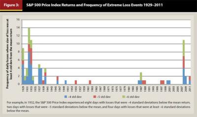
Practice: The investment world is part of a dynamic economic system that has many complicated feedback processes. Multiple extreme events occur within relatively short intervals more often than the theory suggests should be the case. However, it is unlikely that an investor will be able to use this information to consistently make money by betting on extreme events. Between January 1, 1929, and September 13, 2012, an analysis of the daily returns of the S&P 500 Index shows 86 days when the daily return was 4 or more standard deviations below the mean, and 73 days when the daily return was 4 or more standard deviations above the mean. Eighty days are about 0.4 percent of the total days during that period.⁵

For example, Figure 3 shows actual returns for the S&P 500 Price Index, and the years in which extreme market losses occurred. The Cook Pine Capital paper defined an extreme event as a single day market loss that was worse than −4.6 percent, which is equivalent to an occurrence that is 4 or more standard deviations below the mean, if investment returns are assumed to be normally distributed. The historical results for the S&P 500 Price Index contain many more of these extreme events than are predicted by theory (based on a normal distribution). Notice too that the extreme events were clustered together.

Theory: The standard deviation of returns for each asset class and for the portfolio as a whole is an appropriate way for investors to measure risk.

Practice: There are multiple problems with this part of the theory. For example:

• As explained earlier, any model that relies on standard deviation to describe the distribution of returns may substantially underestimate the frequency of extreme events.
• Using standard deviation as a measure of risk implies that any deviation from the mean return is bad—including returns that are higher than the mean return. In reality, investors are worried about losing money; they have no problem if they make more money than they were expecting. Practitioners have tried to address some of the shortcomings of MPT by using measures such as semi-variance to focus on the risk of loss. That is an improvement, but it still leaves other serious problems with the theory.
• Few private investors have a great appreciation for standard deviation as a measure of risk.

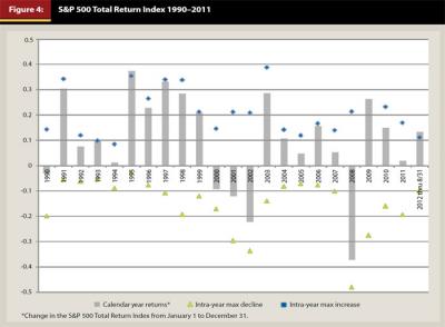
Most portfolio construction techniques use the annual standard deviation of returns for each asset class, but it is more probable that investors tend to react to short-term volatility. For many investors the amount of short-term volatility they experience is much worse than the annual standard deviation of returns seems to imply.

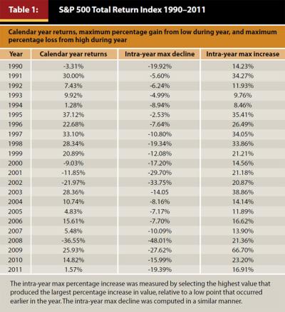
To understand just how much the annual standard deviation of returns masks the amount of volatility that investors actually experience, consider the following statistics using the S&P 500 Total Return Index (SPX) as an example. In Table 1 and Figure 4, the calendar year return measures the change in the S&P 500 Total Return Index from January 1 to December 31. The intra-year maximum decline is the maximum percentage loss an investor experienced during the year, measured between whatever two points during the year produced the largest loss, while always moving forward in time. Thus, the period associated with that loss varies from year to year. The intra-year maximum increase is the maximum percentage gain during the year, measured using a methodology equivalent to the methodology used to determine the maximum decline. The average annual standard deviation of returns was 18.5 percent. It is easy to see the range covered by the maximum decline to maximum increase during most years far exceeded 1 average standard deviation. Small wonder that some individual investors have trouble sleeping at night.

 
Theory: The expected return, standard deviation, and correlations between asset classes remain stable over time.

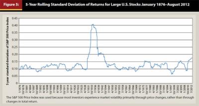
Practice: Nearly all portfolio optimizers are sensitive to changes in expected returns, standard deviations, and correlations between asset class returns. Investment professionals know all of these factors tend to be unstable. For example, Figure 5 shows the five-year rolling average of the standard deviation of returns for U.S. large cap stocks for the period January 1876 to August 2012.Correlations between asset class returns are also unstable. Investors need to be aware that the correlations between asset class returns are constantly changing, and may substantially deviate from the long-term trend line for many decades.
 

One of the keys to managing investment risk is to own a portfolio of assets whose investment returns are independent of one another. In other words, if some asset classes are losing money investors hope to have other asset classes in the portfolio that are showing gains, or at least that all asset classes are not losing money at the same time. That is the goal of diversification. Unfortunately, under conditions of severe market stress, such as occurred in the second half of 2007 and continued through 2008, many investors who thought their portfolios were well diversified were surprised that diversification failed to protect them from losses.

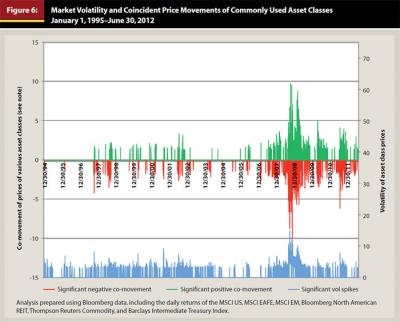
Figure 6 shows price volatility and co-movement of prices for some commonly used asset classes. The asset classes included in the statistics for Figure 6 include: U.S. large capitalization equities, developed international equities, emerging market equities, real estate, commodities, and U.S. government bonds. Figure 6 shows that periods of high market volatility have tended to coincide with periods when the prices of those asset classes have moved in the same direction at about the same time. In other words, during periods of high volatility diversification failed—at least with respect to those commonly used asset classes. Put another way, during periods of high volatility all these asset classes moved together up and down. But, it is only the coincidence of losses that poses a problem for investors.
 

Theory: Investors are indifferent about the liquidity of their investment portfolios. (“Liquid” in this context means readily convertible into cash under a broad range of market conditions and at a price that can be easily determined in advance of the transaction.)

Practice: Most private investors have a very strong preference for liquid investments (Novy-Marx 2004), and they demand compensation in the form of substantially higher expected returns when making an illiquid investment (McCulloch 1975).

In practice, the liquidity problem is addressed in some models by applying an adjustment to the costs or returns of illiquid assets to make them appear to be less attractive. More often, investors or their advisers will simply place constraints on the amount the optimization tool is allowed to allocate to illiquid investments. The constraints are necessary because illiquid asset classes, such as private equity, venture capital, hedge funds, and private real estate funds, are often depicted as having relatively high expected returns and low correlations with other asset classes. Those features appear to make the illiquid asset classes very attractive as portfolio diversifiers. If illiquid assets are not constrained, the mathematics of portfolio optimization may result in a portfolio dominated by illiquid investments. Ironically, individual investors often have been disappointed in the performance of their illiquid assets because those investments have failed to perform as projected. The problems can be traced back to the issues discussed earlier; namely, inability to gain access to top-performing managers, reliance on historical data to project future returns, inadequate diversification, the vintage year problem, etc.

Theory: Any asset class represented in the optimization process can be purchased in any size, without loss of efficiency.

Practice: Private investors face substantial obstacles to obtain efficient access to high-quality investments in many asset classes. This is particularly true of hedge funds, private equity, venture capital, commodities, and private real estate—the asset classes that portfolio optimization models depict as being very important to constructing a diversified portfolio. The problems include, for example, inability to gain access to top-performing managers, high minimum investment amounts, and lack of availability of suitable and attractive investment opportunities when the investor is ready to deploy capital.

Theory: Investors are able to easily rebalance their portfolios at least once a year by moving capital between asset classes to maintain the desired asset allocation.

Practice: Private investors face significant costs, timing problems, and cash flow problems when they seek to rebalance in non-tax-deferred accounts. Investors incur taxes and transaction costs that may cause the investor to indefinitely postpone rebalancing. Annual rebalancing is effectively impossible for many taxable investors within some illiquid asset classes. That portion of the portfolio can be rebalanced only when a liquidity event occurs that frees up capital. Investors typically have no control over the timing of liquidity events in their illiquid investments.

Theory: The performance of the specific investments selected to implement the asset allocation strategy will be closely aligned with the assumptions used to develop the strategy.

Practice: This gap between theory and practice results from the way advisers decide to implement the portfolio recommendations developed with the optimization model. The implementation method selected by many investment firms is not well aligned with the assumptions underlying the strategic asset allocation plan. Many investment firms fill their clients’ portfolios with products whose historical and projected performance bears little resemblance to the performance of the asset class index used during the portfolio optimization process. Many firms recommend active managers whose activities trigger substantial fees, trading costs, and taxes that are not reflected in the index that was used during the portfolio optimization process. The risk that a manager may under-perform relative to the index also is not accounted for. Investment advisers can mitigate this risk by using an appropriate mix of index investment vehicles and active managers.

What Does the Future Hold?

It is obvious the portfolio optimization tools used in the investment world rely upon assumptions that do not fit particularly well in the real world. Yet, these tools are widely used and relied upon by individual investors and advisers as if the underlying assumptions are valid.

For those who find the faults associated with portfolio optimization to be greater than the benefits provided through statistical standardization, the first step is to acknowledge that asset allocation and portfolio construction is mostly an art, not a science. Advisers have an obligation to inform clients of the limitations of the theory. Clients will benefit from being more aware of the substantial gap between asset allocation theory and performance in the real world. Investment success depends upon judgment, skill, and, in the opinion of this author, luck—the latter often showing up as fortuitous timing.

Portfolio optimization tools are useful to assist planners, advisers, and clients in ways to conceptualize the asset allocation problem. But, they should not be relied upon as the primary tool for structuring an investment portfolio. A more reasoned approach is to construct a portfolio around the client’s objectives, informed by the use of statistical tools such as those included in portfolio optimization models. This approach requires a disciplined process that incorporates subjective factors into the analysis. The subjective factors may include a wide range of issues important to the client, including cash flow requirements, risk tolerance, and need for liquidity. This is a more fitting approach for investors than the artificial endeavor of striving to place a portfolio on a theoretical “efficient frontier.”

Clients and portfolio managers following such an approach should ask themselves the following questions:

What measures of risk make sense given the objectives?

It is reasonable to assume the majority of individual investors are primarily concerned with achieving at least a minimum target return necessary to meet their financial goals, while minimizing the risk of significant losses—that is, investors tend to be risk averse. Very few investors understand standard deviation as a measure of risk. Rather than looking at the projected standard deviation of their portfolio, investors and advisers should seek to understand how much the portfolio loss might be under different kinds of extreme conditions. This can be assessed by running simulations, such as Monte Carlo or scenario simulations, using historical data from various periods.

How much does the client have at risk, realistically, and can they afford those risks?

This type of information can be obtained through scenario analyses using historical data. However, clients and advisers should be mindful that the future may reveal even worse scenarios than the typical American has ever experienced.

What is the investment outlook for each major asset class that will be included in the portfolio?

Answering this question requires that the adviser and client have an opinion about the relative pricing of asset classes at the time the portfolio strategy is being formed. Just because a trend is expected (higher inflation) doesn’t mean an asset class, such as commodities, will necessarily perform well if it is already overpriced in the market.

What asset classes make sense in the portfolio?

The assets selected should make sense based on the client’s objectives, tax situation, liquidity requirements, risk policy, and the investment environment that is expected. Investments should be grouped into an asset class based upon an expectation that they will perform in a similar manner, but differently from other asset classes, when it matters most—that is, under conditions of extreme stress in the financial markets. This analysis requires careful thought. Trying to create asset classes based upon statistical analysis alone is not likely to lead to valid conclusions because there is too little data available about extreme events.

What alternative investment scenarios might occur, and how will the asset allocation fare in these scenarios?

Investors should “stress test” their strategies against various environments, asking how each asset class might perform under those circumstances, and how the portfolio as a whole will fare. The client and the adviser should probe for underlying connections between seemingly diverse asset classes to see if there is some common factor that could cause diversification to fail. To do this, the adviser and client may need to collaborate to explore risk factors lurking in the client’s situation. This is especially important for clients who are business owners or investment professionals.

What will drive investment selection?

After a portfolio strategy is established, a key goal is to ensure that each asset class in the portfolio adheres to its assigned mission. Finding managers who may outperform their benchmarks should be secondary. Often, this step gets muddled by investors and advisers who may be lured by performance. A classic example of this is a fixed income manager taking credit risks to beat the benchmark when the manager’s role in the portfolio is to provide downside market protection and to ensure access to liquidity, if needed.

• Advisers and clients also need to incorporate the financial planning aspects of portfolio construction when designing an investment portfolio. This is hard work, which many investment advisers are not well-equipped to do because they lack the necessary time, resources, and training. However, this work is essential to help the adviser develop a deep understanding of the client’s risk tolerance, cash flow requirements, return objectives, liquidity requirements, and tax situation. Specific tasks include: ?Carefully analyzing the client’s balance sheet to identify concentrations of risk, determine available liquidity, and to examine the relationships between assets and liabilities
• Assessing the income tax and transaction costs associated with changing the client’s current portfolio holdings, including: How much will it cost to make changes in the portfolio? (It is important to take into account that the client must pay these costs up front before any of the benefits of portfolio restructuring are realized.) How long will it be before the client recovers these costs? What is the risk that the costs may not be recovered within an acceptable timeframe?
• Analyzing the client’s cash expenditures from today through the end of life expectancy and through estate settlement⁶
• Analyzing the client’s reliable sources of cash flow from earnings, dividends, interest, real estate income, etc.
• Netting reliable cash income against cash requirements to determine the expected amount and timing of cash flow deficits over the entire forecast period
• Developing a plan to fund the cash deficits from the investment portfolio by matching assets with liabilities (the liabilities being the cash flow deficits)
• Measuring the portfolio withdrawal percentage in each year that has a cash flow deficit; withdrawal percentages that consistently exceed 4 percent are probably not sustainable for the long term (Cooley, Hubbard, and Walz 1999)
• Using scenario analysis to determine how large a cash reserve the clients need to have to allow them to feel comfortable sticking with their strategy during challenging investment periods

The search is already on for more useful portfolio optimization tools, both within the field of financial planning and in colleges and universities. Until a model is developed that can incorporate the shortcomings of today’s MPT models, it is important for financial planners to remember that no statistically based tool can adequately substitute for a disciplined and thoughtful approach that considers the practical constraints of the real world and the real needs of investors.

Endnotes

1. Some sources attribute this phrase to Johannes van de Snepscheut, a Dutch computer scientist and educator.
2. As used in this paper, “real estate” includes publicly listed real estate investment trusts (REITs) and private funds that invest in various kinds of real estate, and “commodities” refers to publicly listed funds and private funds that invest primarily in energy, agricultural products, industrial metals, and other raw materials.
3. Manager selection risk is the risk associated with selecting the wrong manager for an asset that requires active management. Manager selection risk is very high for hedge funds, private equity, private real estate, and venture capital funds.
4. Some portfolio optimization models use factor analysis to reduce the number of variables that must be forecast. It is possible, for example, that variations in three or four observed variables mainly reflect the variations in fewer unobserved variables. Factor analysis searches for such joint variations in response to unobserved latent variables.
5. Ballentine Partners, LLC table available at www.ballentinepartners.com/914785.pdf.
6. This analysis calls for the creation of various scenarios, including both spouses living well beyond actuarial life expectancy, the primary income-earning spouse dying early, disability of either spouse, loss of income by the primary income-earning spouse, etc.

References

Cook Pine Capital. 2008. “Study of Fat-tail Risk,” Google docs.

Cooley, Philip, Carl Hubbard, and Daniel Walz. 1999. “Sustainable Withdrawal Rates from Your Retirement Portfolio.” Journal of Financial Counseling and Planning 10, 1: 40-50.

Lhabitant, Francois-Serge, and Michelle Learned. 2002. “Hedge Fund Diversification: How Much is Enough?” FAME Research Working Paper 52 (July): http://ssrn.com/abstract=322400 or http://dx.doi.org/10.2139/ssrn.322400.

Mandelbrot, Benoit. 1963. “The Variation of Certain Speculative Prices.” Journal of Business 36 (October): 394–419.

Mandelbrot, Benoit and Richard Hudson. 2004. The (Mis)behavior of Markets: A Fractal View of Risk, Ruin, and Reward. New York, NY: Basic Books.

McCulloch, J. 1975. “An Estimate of the Liquidity Premium.” Journal of Political Economy 83, 1: 95–119.

Novy-Marx, Robert. 2004. On the Excess Returns to Illiquidity. Center for Research in Security Prices, Graduate School of Business, University of Chicago.

Rivera, Peter. 2013. “Theory & Reality Risk Management,” www.theoryandreality.com/resources/rm_faq1.html.

Taleb, Nassim. 2007. “Black Swans and the Domains of Statistics.” The American Statistician 61, 3: 198–200.