Tax-Efficient Retirement Withdrawal Planning Using a Comprehensive Tax Model

Journal of Financial Planning: April 2012

Alan R. Sumutka, CPA, is an associate professor of accounting at Rider University in Lawrenceville, New Jersey, and the owner of Alan R. Sumutka, CPA. (sumutka@rider.edu)

Andrew M. Sumutka, Ph.D., is an assistant professor of management at York College of Pennsylvania in York, Pennsylvania. (asumutka@ycp.edu)

Lewis W. Coopersmith, Ph.D., is an associate professor of management sciences at Rider University, and provides consulting to industry and government on forecasting and market dynamics. (coopersmith@rider.edu)

Executive Summary

• A highly precise comprehensive tax model that calculates state and federal income taxes (including the AMT, the impending 3.8 percent Medicare tax, and Medicare premiums) is used to evaluate 15 withdrawal strategies (including variations) and several tax strategies for tax efficiency (the strategy that maximizes the final total account balance over a planning horizon).
• Base model results show that the tax-efficient strategy (TD_D) is achieved by long-term income stability and characterized by low withdrawal rates early in retirement, sequenced as follows: tax-deferred assets up to tax deductions, the rapid depletion of taxable assets, tax-free assets, and tax-deferred assets, preserved throughout the planning horizon. This strategy produces the highest final total account balance, gained through an average 4.5/6.6 percent pre-/post-RMD withdrawal rate, respectively.
• Variable analysis confirms the tax efficiency of the TD_D strategy and suggests it should be the new “common rule” (CR). Using tax-deferred assets to fill the 10 percent tax bracket (TD₁₀) or the current CR (sequentially deplete taxable, tax-deferred, tax-free accounts) produces optimal results in limited cases and with minor benefits. The arbitrary use of the current CR results in significantly lower balances. Withdrawing tax-deferred assets beyond TD₁₀ or tax-free assets before taxable assets is tax-inefficient.
• Strategies that produce the highest final total account balance rarely produce the lowest total taxes. Several common tax minimization and estate planning strategies do not produce optimal results.

A prospective retiree’s portfolio may hold investments in three accounts, each affected differently by tax laws:

• Tax-deferred accounts (including traditional IRAs and 401(k) plans) in which contributions and investment earnings are tax-deferred and withdrawals are taxed as ordinary income
• Taxable accounts (for example, brokerage accounts) in which some earnings and withdrawals (including qualified dividends and long-term capital gains) are taxed at favorable tax rates and other earnings (for example, interest) are taxed as ordinary income
• Tax-free accounts (for example, Roth IRAs) in which earnings and withdrawals are not taxed
  Upon retirement, different withdrawal sequences (the order and amount withdrawn annually from each account type) produce different tax and wealth results. Slott opines (see Buttell 2010), “The typical financial adviser gets into the business and thinks, ‘My job is to make people money.’ But when taxes are reaching the level that we’re seeing now, and going to see, taxes become the single biggest factor that will determine how much of their money … they will actually keep.” Because taxes in retirement are an important determinant of portfolio longevity, tax-efficient withdrawal plans are critical.

As in Coopersmith and Sumutka (2011), we consider a withdrawal plan tax efficient if it includes all of the following:

• Consideration of more than one annual withdrawal strategy over a retirement horizon—each strategy differs by the sequence of withdrawals from different accounts, and each account has a different tax treatment
• A realistic calculation of taxes for each strategy
• Selection of the best strategy with respect to some performance measure (for example, final total account balance)
  Literature Review

To develop a tax-efficient withdrawal strategy, prior research considers varying degrees of tax precision. Ragsdale, Seila, and Little (1994) use a linear programming (LP) model with basic tax provisions (for example, required minimum distributions (RMDs)) to evaluate tax-deferred account withdrawals. Spitzer and Singh (2006) use a flat tax rate to evaluate withdrawals from two accounts. They conclude that the account with the lowest expected return is best depleted first. Bernachhi (2008) considers Social Security taxation, capital gains rates, RMDs, progressive tax rates, and taxable and tax-deferred accounts to determine an optimal account mix at the start of retirement.

Much research applies to the “common rule” (CR) that taxable assets are best used first and tax-deferred assets used last to permit tax-sheltered growth in tax-deferred and tax-free accounts. Reichenstein (2006) considers three retirement accounts, RMDs, progressive tax rates, and a 15 percent long-term capital gains rate, and agrees with the CR. However, excessive tax-deferred account growth can create unnecessary RMDs, possibly taxed at higher tax rates. Withdrawing tax-deferred assets prior to or in excess of RMDs potentially transforms ordinary income into tax-free income (if the added withdrawal is offset by tax deductions) or lower taxed income (if the withdrawal is taxed at a lower than anticipated future tax bracket), reduces future RMDs, and permits further growth in tax-free assets. Reichenstein (2006, 2008) recommends first using tax-deferred assets to fill “low tax brackets” (the 10 percent tax bracket) and the 15 percent bracket for wealthier individuals before RMDs begin.

Using tax-deferred and Roth IRA accounts and progressive tax rates, Horan (2006a, 2006b) confirms the benefit of a 15 percent bracket fill, but adds that wealthier investors gain from 25 percent and 28 percent bracket fills followed by withdrawals from Roth IRAs. Spitzer (2008) uses taxable and tax-deferred accounts and Social Security tax calculations to assess the impact of RMDs on four cases. He concludes that transferring excess RMDs to a taxable account is an effective “coping strategy.” Coopersmith and Sumutka (2011) use an LP model that includes taxable and tax-deferred accounts and basic tax provisions (for example, 85 percent of Social Security is taxed, RMDs, progressive tax rates). They conclude that for various scenarios, the LP model-determined withdrawals from the tax-deferred account before the taxable account maximize the final total account balance.

Other research and policy recommendations address tax minimization. Van Harlow and Feinschreiber (2007) develop five guidelines for a personal withdrawal hierarchy. They proffer, “There is one common, continuous ‘tactical’ goal that all retirees share: minimizing the impact of taxes on their incomes.” Guyton (2010) suggests that a withdrawal policy statement might contain a goal to “minimize the long-term income taxation of our withdrawal income.” Using limited examples, Bernacchi (2008) and Coopersmith and Sumutka (2011) find that tax minimization is not always tax efficient.

If bequest maximization is desired, Reichenstein (2006) cautions that selling highly appreciated taxable assets before death forfeits the basis step-up. Shynkevich (2010) considers taxable and tax-deferred accounts, RMDs, and flat income and capital gains rates. He concludes that in community property states, the decedent earns a 100 percent basis step-up, which justifies postponing taxable account withdrawals until after the death of a spouse, and provides a hedge against the probable higher income-tax rates of the survivor.

Research Design

A unique aspect of this paper is to evaluate the tax efficiency of various withdrawal and tax strategies through the use of a comprehensive tax model (CTM) that calculates income taxes as completely and accurately as tax preparation software. We expand Horan’s research design (2006b) and compare 15 withdrawal strategies to determine the final total account balance and total taxes in retirement:

• Three naïve strategies: after RMDs are satisfied from the tax-deferred account, the account balances are depleted as follows: (A) tax-free, taxable, tax-deferred; (B) tax-deferred, taxable, tax-free; or (C) taxable, tax-deferred, tax-free (the CR)
• Six informed strategies: (D) draw from the tax-deferred account in the amount of tax deductions (the greater of the standard or itemized deductions and personal exemptions) and RMDs (when greater than tax deductions), followed by the sequential depletion of the taxable, tax-free, and tax-deferred accounts. The other five informed strategies follow the same pattern, but the initial tax-deferred withdrawal is increased to fill to the top of the different tax brackets: (E) 10 percent, (F) 15 percent, (G) 25 percent, (H) 28 percent, and (I) 33 percent.
• Six additional informed strategies (J through O): these mirror the first six informed strategies, except that the initial tax-deferred withdrawal is followed by the sequential depletion of tax-free, taxable, and tax-deferred accounts.
  Hereafter, we denote the tax-bracket fill strategies by the amount of tax-deferred assets that fill a tax bracket. For example, TD_D represents a fill up to tax deductions; TD₁₀ is a fill to top of the 10 percent tax bracket, etc.

In all strategies, specified financial needs (living expenses, itemized deductions, and taxes) are satisfied by Social Security and withdrawals. All interest and dividends are reinvested. Withdrawals occur on the first day of the year. If RMDs exceed financial needs, the excess tax-deferred amount is transferred to the taxable account at the beginning of the year.

Our CTM, which incorporates 2011 federal tax laws,¹ provides a high degree of tax precision. It:

• Includes three accounts: tax-deferred, taxable, and tax-free²
• Calculates state³ and federal income taxes, including the regular tax, the alternative minimum tax (AMT),⁴ the impending 3.8 percent Medicare health insurance tax on net investment income (MHI tax)⁵ (Fava and Rubin 2011), and means-tested Medicare Part B health insurance premiums (MHI premiums),⁶ which some tax planners (Meeting, Cornick, and Alvis 2010) and the authors regard as a tax
• Calculates and/or includes in the calculation the actual amount of Social Security subject to tax⁷ and RMDs,⁸ CTM-determined itemized deductions for state income tax and MHI premiums, Internal Revenue Service (IRS) itemized deduction averages for others,⁹ the larger of the standard deduction¹⁰ or itemized deductions, personal exemptions,¹¹ and the favorable (0 or 15 percent) tax treatment for qualified dividend income (QDI) and long-term capital gains (LTCG)¹²
• Considers the dynamic interaction among tax calculations; for example, lower tax-deferred asset withdrawals prior to RMDs produce higher RMDs, which: (1) increase future retirement income, Social Security subject to tax, adjusted gross income (AGI), and taxable income (TI), (2) reduce the amount of itemized deductions and the favorable tax treatment for QDI and LTCG, and (3) trigger the AMT, the MHI tax, and higher MHI premiums.
  The comparative performance measure is the final total account balance at the end of a 30-year planning horizon; the “best” plan is referred to as the optimal withdrawal strategy (OWS). We are indifferent about the composition of the final total account balance.¹³

The base model considers a married couple who retire in 2013 at age 66. They have $2 million in retirement savings (70 percent in tax-deferred accounts, 20 percent in taxable accounts, and 10 percent in tax-free accounts). Each account consists of the same stock/bond asset allocation (to permit unencumbered withdrawal from any account despite market volatility) and earns a 6 percent rate of return (ROR) (1 percent in QDI, 1 percent in non-QDI or interest, and 4 percent in appreciation). First-year living expenses (before itemized deductions and taxes) are $80,000, which is partially offset by $30,000 in Social Security, resulting in a $50,000 withdrawal, or a 2.5 percent basic withdrawal rate. However, withdrawals are increased by itemized deductions (including a 3 percent state income tax and MHI premiums) and federal income taxes (the regular tax, the AMT, and MHI tax) resulting in a total withdrawal rate of 4.5 percent. A 2 percent inflation rate applies to expenses and inflation-adjusted amounts (for example, Social Security, standard deduction, tax brackets). Fifty percent of the taxable account withdrawals are LTCG. Thirty years of withdrawals are calculated, ending when the couple reaches age 96.

Variations from the base model (in bold) are evaluated individually and include:

•Asset location (the percent of initial assets in each account) by percent tax-deferred/percent taxable/percent tax-free: 90/10/0, 80/15/5, 70/20/10, 60/25/15, 50/30/20, 40/35/25, 30/40/30, 20/45/35, 10/50/40, 0/55/45
•Initial account balance: $1 million, $2 million, $3 million, $4 million, $5 million, $6 million, $7 million, $8 million
•Social Security income: $0, $10,000, $20,000, $30,000, $40,000, $50,000, $60,000
•Living expense basic withdrawal rate (pre-itemized deductions and taxes) as a percentage of initial account balance: 5.5 percent, 4.5 percent, 3.5 percent, 2.5 percent, 1.5 percent, 0.5 percent, N/A (Social Security only)
•Percentage of withdrawals that are LTCG: 90 percent, 75 percent, 50 percent, 25 percent, 0 percent
•ROR: 4 percent, 5 percent, 6 percent, 7 percent, 8 percent
•Composition of 6 percent base model ROR by QDI percentage/non-QDI percentage/appreciation percentage: 2/2/2, 1/2/3, 2/1/3, 1/1/4, 0/0/6
•Inflation rate: 5 percent, 4 percent, 3 percent, 2 percent, 1 percent
•State income-tax rate: 5 percent, 4 percent, 3 percent, 2 percent, 1 percent, 0 percent
•Percentage of average itemized deductions: 0 percent, 50 percent, 100 percent, 150 percent, 200 percent
Base Model Results

Table 1 shows the results of the 15 withdrawal strategies. There is a clear benefit of first withdrawing some tax-deferred assets and then using taxable assets. This provides sufficient freedom for the tax-free and tax-deferred accounts to grow tax-free. The OWS (strategy D) employs TD_D and has a final total account balance of $1.61 million. Strategy E uses TD₁₀; its balance is only $4,000 less than TD_D. Using TD_D and TD₁₀, but reversing the order of the second and third withdrawals to tax-free followed by taxable assets (strategies J and K, respectively) produces the third- and fourth-best results. However, if tax-deferred assets fill beyond TD₁₀, results suffer regardless of subsequent withdrawal sequences. None of the naïve withdrawal strategies (A, B, and C) are tax efficient; the CR produces the sixth-best result.

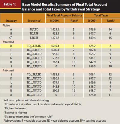
Table 2 illustrates that accurate tax calculations are critical to determining tax efficiency. In various strategies, the federal regular tax, AMT, MHI tax, MHI premiums, and state taxes reach $588,000, $21,000, $3,000, $150,000, and $110,000, respectively. Ignoring all taxes understates total withdrawals needed by $625,000 in the OWS and $849,000 in the highest-taxed strategy C. If only the federal regular tax is considered, the expense understatement is $221,000 in the OWS and $261,000 in strategy C.

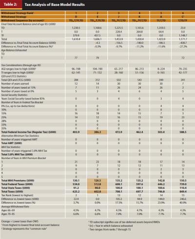
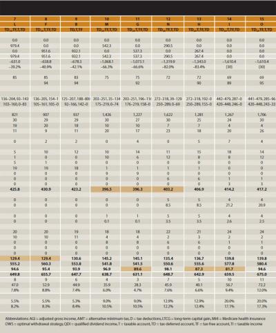
The two best strategies, D and E, are analyzed in detail in the left-most columns of rank 1 and 2 in Table 2. These two strategies illustrate that a tax-efficient strategy for the base model depletes the taxable account quickly and maintains the stability of AGI and TI throughout the planning horizon. Adverse tax consequences are thus avoided as income rises, but not necessarily with lower taxes in a particular year or years. Over the planning horizon for strategy D (TD_D), AGI increases gradually from $96,000 to $198,000 (a $102,000 variance) and TI from $62,000 to $141,000 (an $89,000 variance). Similarly, strategy E (TD₁₀) has AGI and TI variances of only $86,000 and $61,000, respectively. No other strategies produce such consistency, and neither strategy triggers the AMT or MHI tax. By first using TD_D, future RMDs are reduced and ordinary income is transformed to tax-free income because tax deductions are satisfied from tax-deferred asset withdrawals. Although taxable assets usually generate tax-favored income, QDI and LTCG are still taxed. Depleting the taxable account quickly (after 12 and 14 years, respectively) results in a low QDI and LTCG total, taxed only in 7 of the 12 years for the OWS.

Importantly, throughout the planning horizon, each strategy maintains balances in both the tax-deferred (which later offsets tax deductions) and tax-free account (for continuous tax-sheltered growth in both accounts). Interestingly, the maximum 85 percent of Social Security is always taxed, and TI is never taxed in the 0 or 10 percent tax brackets. A key distinction between the top two strategies is that TD_D has modestly better income stability. It is taxed in the 15 percent tax bracket for 16 years and the 25 percent tax bracket for 14 years; it is in the lowest MHI premium bracket for 21 years and the second-lowest bracket for 9 years. In contrast, TD₁₀ is taxed in the 15 percent tax bracket for 18 years, the 25 percent tax bracket for 12 years, the lowest MHI premium bracket for 23 years, and the second-lowest bracket for 7 years. These slight variations reduce the average total withdrawal rate prior to RMDs to 4.5 percent in TD_D and 4.7 percent in TD₁₀. Both strategies average a 6.6 percent total withdrawal rate after RMDs begin.

For strategies ranked 3 (strategy J), 4 (strategy K), and 5 (strategy A) in Table 2, tax-free assets are withdrawn before taxable assets. Strategies J and K mirror the top two strategies by employing TD_D and TD₁₀, respectively. Naïve strategy A withdraws no tax-deferred assets initially. All of these strategies produce tax reductions in individual components of the tax calculation. For example, by taking tax-free assets before taxable assets, strategy J produces four years in which less than 85 percent of Social Security is taxed; strategy K produces the most stable number of years in the 15 and 25 percent income-tax brackets (15 years each).

Strategies J and K generate final total account balances of 10 percent to 12 percent less than the OWS. They deplete tax-free assets faster than most other strategies (by age 70 and 71, respectively) and never deplete taxable assets. This produces higher amounts of QDI and LTCG (taxed at 15 percent for 26 and 24 years, respectively), which increase AGI and TI, their variances, and the number of years MHI premiums are taxed in the second MHI bracket. Similarly, naïve strategy A (which withdraws all tax-free assets first) produces three years in which less than 85 percent of Social Security is taxed, a lower amount of QDI and LTCG, and four years of income taxed in the 0 percent bracket. However, it also has the earliest depletion of tax-free savings (age 68) and produces higher AGI and TI amounts and variances, 19 years of income taxed in the 25 percent bracket, and 2 years in the third MHI premium bracket. The amplified income volatility and life-long retention of taxable assets create three of the highest tax liabilities among all strategies (ranks 13, 12, and 14, respectively).

CR (strategy C) produces the sixth-highest final total account balance, which is less than the OWS by $439,000 (27 percent). It depletes taxable assets before any strategy (age 72), produces the lowest amount of QDI and LTCG (taxed in only two of seven years), and results in four years in which less than 85 percent of Social Security is taxed. However, by using no tax-deferred assets until taxable assets are depleted, CR forfeits the advantage of offsetting ordinary income with tax deductions. Instead, tax deductions offset tax-favored QDI and LTCG, which causes further AGI/TI disadvantages: the highest number of years (23) in the 25 percent tax bracket, three years in the third-highest MHI premium bracket, and the highest tax burden of any strategy.

The nine lowest-ranking strategies have a common feature: initial withdrawals exceed TD₁₀. This results in final account balances less than OWS by $631,000 (39 percent) to $1.6 million (100 percent). These strategies also produce volatile AGI and TI swings and many years of low or no tax on/for QDI and LTCG, Social Security, and MHI premiums. Either TD₂₅ strategy even produces the third- and fourth-least total taxes. Conversely, the income volatility causes several very high tax years. For example, the accelerated tax-deferred bracket fill reduces its tax-deferred growth potential and prolongs the depletion of the taxable account, which causes the highest amounts of QDI and LTCG and triggers the AMT, MHI tax, and the highest number of years in the third-highest MHI premium bracket.

Table 2 illustrates that tax minimization often is a worthy goal; the two best strategies produce the lowest taxes. However, tax minimization is not always tax efficient. For example, the OWS generates more taxes than the second-ranked strategy ($625,000 vs. $603,000); other strategies with high total taxes (tax ranks 13, 12, 14, and 15) have high final total account balances (strategy ranks 3, 4, 5, and 6, respectively). Also, withdrawal strategies focused on year-to-year tax avoidance often sacrifice long-term income stability and final total account balances. For example, strategies with low total taxes (tax ranks 4, 3, and 5) have low final total account balances (strategy ranks 10, 11, and 13, respectively).

A withdrawal strategy that uses tax-deferred assets to fill to the current or projected tax bracket to reduce future RMDs is not necessarily tax efficient. For example, in strategy D, TD_D (the OWS) is taxed in the 15 and 25 percent tax brackets throughout retirement. If TD₁₅ and TD₂₅ strategies (F and G) are used, the final total account balance is significantly lower (by $659,000 and $1.073 million, respectively).

Estate planning strategies, which seek the highest taxable asset balance (to receive a basis step-up) or tax-free asset balance (to “stretch” the benefit to future generations) and the lowest tax-deferred balance (to avoid ordinary income taxation) at the end of the planning horizon, are not tax efficient. As illustrated by strategies ranked 6 through 13, a retiree sacrifices from $439,000 to $1.343 million (27 percent to 83 percent, respectively) over a lifetime for these benefits.

The results highlight that no strategy produces only one income tax bracket throughout the planning horizon, which complicates research that uses after-tax account values based on a single projected tax bracket.

Variable Analysis Results

Tables 3 and 4 illustrate that in most cases the variable analysis agrees with the base model results: strategies D and E, which employ TD_D and TD₁₀, respectively, usually are tax efficient and produce differences between each other’s final total account balances of less than 3.2 percent, or $28,000. In only three circumstances CR (strategy C) is superior but leads strategy D by no more than 1.5 percent, or $38,000.

Table 3 illustrates the impact of changes in asset locations. An original portfolio of $2 million composed of 90 percent tax-deferred assets, 10 percent taxable assets, and no tax-free assets creates considerable ordinary income, no tax-free asset growth, and thus the lowest final total account balance ($980,000). However, as the mix shifts from tax-deferred to tax-favored taxable and tax-free assets, the final total account balance steadily increases to $2.605 million, which demonstrates the benefit of skewing the asset mix at the start of retirement to favor taxable and tax-free accounts.

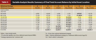
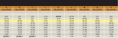
With 50 percent taxable and 40 percent tax-free assets, CR depletes the high level of taxable assets most rapidly and produces the highest final total account balance. As the taxable and tax-free amounts decrease, TD_D becomes the OWS. However, at the lowest levels of taxable (10 and 15 percent) and tax-free (0 and 5 percent) assets and the highest levels of tax-deferred assets (90 and 80 percent), TD₁₀ reduces future RMDs and produces the highest final total account balances. When there are no tax-free assets, strategies D through I and J through O draw in the same sequence (tax-deferred, taxable, and tax-deferred), so the results are identical. Similarly, when there are no tax-deferred assets, the results of strategies A and J through O and B through I are identical.

Table 3 also illustrates that any strategy that considerably delays the depletion of taxable assets or curtails the growth of tax-free and tax-deferred assets is never the only OWS. These unfavorable results occur for:

• Naïve strategy A when the tax-free account is fully depleted first
• Strategies J through O, which first deplete the tax-free account and fill various tax brackets
• Naïve strategy B when the tax-deferred account is fully depleted first
• Strategies F through I used to fill beyond the 10 percent tax bracket

Therefore, the results of these strategies are omitted from Table 4.

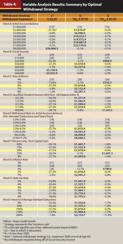
Table 4, Panel A shows that as initial account balances increase (from $1 million to $8 million), final total account balances increase to $26.968 million. In most scenarios, TD_D is optimal. However, at $8 million of initial assets, RMDs cause taxation at the highest brackets. Thus, CR is best because it reduces the taxable account early to provide some tax savings; however, the final total account balance difference is only $27,000 more than TD_D. At $1 million of initial assets, the withdrawal rate is unsustainable, regardless of strategy.

Table 4, Panel B illustrates that changes in Social Security (from $0 to $60,000) produce results similar to asset location variations. At the highest levels of Social Security ($50,000 and $60,000), fewer withdrawals are necessary, and account balances swell. CR depletes the high levels of taxable assets most swiftly and never uses tax-free assets. However, as Social Security decreases to $40,000 and $30,000, TD_D is optimal. As Social Security further declines to $20,000, TD₁₀ produces the highest final total account balance. At the lowest Social Security amounts ($10,000 and $0), all accounts are exhausted before the end of the planning horizon.

Table 4, Panel C illustrates the effect of changes in ROR. At 4 percent, no strategy is sustainable beyond 24 years. However, as the ROR increases from 5 percent to 8 percent, the final total account balances increase from $316,000 to $5.248 million, respectively. For most RORs, TD_D is optimal. Similar to variations in Social Security, TD₁₀ is optimal only at lower projected final total account balances.

Table 4, Panel D illustrates the impact of changes in ROR components. The lowest final total account balance results when the base model 6 percent ROR is earned equally among QDI, non-QDI, and appreciation (2 percent each). However, as the taxable component decreases and the nontaxable part increases, the final total account balances also rise. These results support Reichenstein’s (2008) recommendations to hold tax-inefficient assets (for example, interest-bearing assets) in tax-deferred or tax-free accounts and tax-efficient assets (for example, individual stocks) in taxable accounts. With a 6 percent ROR composed entirely of appreciation, the taxable account grows tax-free, with 50 percent of withdrawals subject to LTCG. This plus the apparent buildup in tax-deferred assets favors TD₁₀. All other results indicate TD_D.

Table 4, Panel E shows the impact of changes in withdrawal rates. For total rates between 7.6 percent and 5.6 percent, no strategy is sustainable. However, as the total withdrawal rate decreases from 4.5 percent to 1.2 percent, the final total account balance increases from $1.610 million to $8.949 million by using TD_D. Significantly, the base model considers a conservative 6 percent ROR composed of only 1 percent QDI, 1 percent non-QDI, and 4 percent annual appreciation, yet the 4.5 percent withdrawal rate exceeds the often quoted 4 percent safe withdrawal rate (see Salter and Evensky 2008). Even a slightly higher return increases the withdrawal rate beyond 4.5 percent.

The results in Table 4, Panel F seem counterintuitive: as the percent of LTCG increases (from 0 to 90 percent), the final total account balance decreases. However, considering that LTCG results from taxable asset withdrawals, the result is rational. If taxable assets are sold at no gain, there is no tax impact, but the asset balance decreases by the withdrawal amount. However, as LTCG increases, taxes and withdrawals increase (albeit the gain is taxed favorably) and the final total account balance decreases. Models that ignore the LTCG treatment overstate the final total account balance. Of course, when compared with the same percentage withdrawal of only short-term capital gains, a withdrawal composed of only LTCG produces lower taxes and a higher final total account balance. We observe TD_D is optimal under all variations, with the exception of taxable withdrawals composed of 25 percent LTCG, which indicates a TD₁₀ fill—nearly identical in final total account balance to TDD (an insignificant difference of $2,000).

Table 4, Panels G, H, and I illustrate the effect of varying expenses. Of course, as expenses decrease (as a result of lower inflation, state tax rates, or federal taxes because of higher itemized deductions), final total account balances increase. In all variations, TD_D is optimal, except at 3 percent inflation where TD₁₀ is better.

As noted previously, the AMT, MHI tax, and MHI premiums potentially cause adverse tax consequences. However, in most cases, a tax-efficient withdrawal strategy does not trigger them, or mitigates their impact. An online appendix at www.FPAnet.org/Journal/0412Appendix highlights that a plausible risk exists only when a variable is likely to create large account balances (for example, high Social Security, ROR, initial account balance, or low withdrawal rates). It also confirms that minimizing taxes does not always maximize the final total account balance, as none of these optimal results generate the lowest taxes. In unreported results, the OWS produces the lowest total taxes only when the average itemized deductions are doubled to 200 percent and in several asset location shifts.

Conclusions

We contribute to retirement withdrawal research by using a highly precise CTM that calculates all state and federal income taxes, including the AMT, MHI tax, and MHI premiums to evaluate the tax efficiency of 15 withdrawal strategies applied to a base model, as well as a wide range of variations around the base model, plus several tax strategies.

Our results are in basic agreement with prior research regarding the benefits of accelerating the withdrawal of tax-deferred assets beyond RMDs. Key implications related to the base model results are:

• Tax efficiency is usually achieved by maintaining long-term income stability to avoid the volatility in AGI and TI that leads to the loss of itemized deductions and tax-favored QDI and LTCG treatment, and triggers higher federal and state income taxes and MHI premiums, the AMT, and MHI tax
• The OWS is characterized by low withdrawal rates early in retirement, sequenced as follows: TD_D, the rapid depletion of taxable assets, tax-free assets, and lastly tax-deferred assets, preserved in amounts sufficient to be offset by tax deductions throughout the planning horizon. Despite using conservative base-model assumptions, the OWS creates a final account balance of $1.61 million gained through an average 4.5 percent pre-RMD withdrawal rate and an average 6.6 percent post-RMD withdrawal rate. \

The variable analysis confirms the tax efficiency of the TD_D withdrawal strategy:

• TD₁₀ is optimal in limited cases, with only small benefits (less than 3.2 percent or $28,000) over TD_D
• Withdrawing tax-deferred assets beyond TD₁₀ is not tax efficient
• Contrary to popular belief, CR is tax efficient only at high levels of initial taxable assets (for example, 45 to 55 percent), initial account balances (for example, $8 million), and/or Social Security (for example, $50,000 and $60,000). Compared with TD_D, the advantage is less than 1.5 percent or $38,000. The arbitrary use of CR can be perilous, with results from 20 percent to 100 percent less than the OWS.
• Any strategy in which tax-free assets are withdrawn before taxable assets is not optimal
  The results suggest the new “common rule” should be TD_D: first withdraw tax-deferred assets to fill up to tax deductions.

The results indicate that a withdrawal goal to produce the maximum final total account balance and the lowest total taxes in retirement is usually unattainable. Although the OWS provides relatively low taxes and/or avoids some taxes (especially the AMT and MHI tax), usually the greater wealth generated by the OWS causes higher taxes; inefficient strategies create lower wealth, which generates lower taxes. We observe that tax inefficiency results from common practices such as:

• Reducing the short-term taxation on certain income items (for example, Social Security, QDI, LTCG)
• Using tax-deferred assets to fill to a current or projected tax bracket to reduce future RMDs
• Delaying the use of taxable assets to obtain a future basis step-up
• Accelerating the use of tax-deferred assets to avoid taxes to heirs

A CTM provides an accurate estimate of income taxes, financial needs, final total account balances, and tax brackets, especially at high levels of wealth, at which the AMT, MHI tax, and MHI premiums are onerous. The model also assists tax-bracket-based planning decisions (for example, traditional vs. Roth IRA contributions, or Roth conversions). It can be modified for federal tax law changes, tailored for specific state income tax calculations, and used for “what if” analysis. It is anticipated that projections and strategies are revised annually.

Using a CTM, future research may incorporate Monte Carlo simulations, assess the tax efficiency of withdrawal strategies when combinations of variables are considered (for example, accounts possess different RORs), introduce annuities, and adjust living expenses for changes attributed to increasing age or declining health. 

Endnotes

1. We assume the “Bush tax cuts” are extended beyond 2012.
2. Only Roth IRAs are considered.
3. State taxes are a percentage of the CTM-computed federal taxable income.
4. The AMT adjusts the federal regular tax for different AMT laws. In 2011 a couple gets a $74,450 exemption, which phases out at high income levels. We assume this “patch” increases 3 percent annually.
5. The MHI tax is effective January 1, 2013. Generally, for a nonworking couple, it is 3.8 percent of the lesser of (1) net investment income (including interest, dividends, capital gains) or (2) modified adjusted gross income (MAGI) less a $250,000 (non-inflation-adjusted) threshold. For most retirees, MAGI and AGI are identical.
6. MHI premiums are based on MAGI (two years prior to assessment), which we assume is $200,000 in 2011 and 2012. In 2011 the annual premiums for a couple with MAGI between $170,000 and $214,000 are $3,876. The post-2019 inflation adjustments to the five MAGI brackets are ignored.
7. The amount of Social Security subject to tax ranges from 0 to 85 percent.
8. RMDs apply to tax-deferred accounts and generally begin at age 70½.
9. The IRS reports annual average itemized deductions several years after a filing year. The 2008 averages for AGI from $100,000 to $200,000 are medical: $9,269; state taxes: $10,798; and charitable contributions: $3,757 (Commerce Clearing House 2008). We “gross up” the medical expenses, and assume the couple incurs 90 percent of medical expenses, 50 percent of state taxes, and 100 percent of charitable contributions. All amounts are inflated to 2013. The remaining medical expenses and state taxes are CTM-generated. Medical expenses are deductible in excess of 7.5 percent (10 percent after 2016) of AGI. No other itemized deductions are considered.
10. The standard deduction for a couple is $13,900.
11. The personal exemptions for a couple are $7,400.
12. QDI and LTCG rates are 15 percent if income is taxed at a higher than 15 percent rate and 0 percent if income is taxed at 15 percent or lower.
13. A balance at death may comprise (1) taxable assets, providing a basis step-up, or (2) tax-deferred assets, subjecting it to income tax. However, such targeted balances are a matter of preference. For example, retaining tax-deferred assets is wise if the retiree is in a higher tax bracket than the heir (who pays at a lower rate on an inherited IRA), has charitable intentions, anticipates high medical expenses (including assisted or nursing care, where these normally deductible expenses shelter ordinary income) (Reichenstein 2008), or prefers the highest account balance for unexpected future needs.

References

Bernacchi, Ben T. 2008. “Determining the Proper Starting Balance for Taxable and Tax-Deferred Savings at Retirement.” Journal of Financial Planning 21, 7: 56–62.

Buttell, Amy E. 2010. “Ed Slott on Roth IRAs, Automatic IRAs, and Retirement Planning.” Journal of Financial Planning 23, 10: 20–24.

Commerce Clearing House. “Average Itemized Deductions.” http://www/cch.com/wbot2011/029AvgItemizedDeductions.asp.

Coopersmith, Lewis W., and Alan R. Sumutka. 2011. “Tax-Efficient Retirement Withdrawal Planning Using a Linear Programming Model.” Journal of Financial Planning 24, 9: 50–59.

Fava, Karl L., and Kenneth L. Rubin. 2011. “Planning for the New 3.8% Medicare Tax on Unearned Income.” Tax Adviser 42, 7: 472–475.

Guyton, J. T. 2010. “The Withdrawal Policy Statement.” Journal of Financial Planning 23, 6: 41–44.

Horan, Stephen M. 2006a. “Optimal Withdrawal Strategies for Retirees with Multiple Savings Accounts.” Journal of Financial Planning 19, 11: 62–75.

Horan, Stephen M. 2006b. “ Withdrawal Location with Progressive Tax Rates.” Financial Analysts Journal 62, 6: 77–87.

Meeting, David T., Michael Cornick, and Charles Alvis. 2010. “Medicare Part B Premiums: A Hidden Income Tax.” CPA Journal 80, 12: 42–45.

Ragsdale, Cliff T., Andrew F. Seila, and Philip L. Little. 1994. “An Optimization Model for Scheduling Withdrawals from Tax-Deferred Retirement Accounts.” Financial Services Review 3, 2: 93–109.

Reichenstein, William. 2006. “Tax-Efficient Sequencing of Accounts to Tap in Retirement.” Trends and Issues, TIAA-CREF Institute (October).

Reichenstein, William. 2008. In the Presence of Taxes: Applications of After-Tax Asset Valuations. Denver: FPA Press.

Salter, John R., and Harold Evensky. 2008. “Calculating a Sustainable Withdrawal Rate: A Comprehensive Literature Review.” Journal of Personal Finance 6, 4: 118–137.

Shynkevich, Andrei. 2010. “Marital Status and State of Residence as Determinants of the Optimal Withdrawal Strategy.” Financial Services Review 19, 3: 203–226.

Spitzer, John J. 2008. “Do Required Minimum Distributions Endanger ‘Safe’ Portfolio Withdrawal Rates?” Journal of Financial Planning 21, 8: 40–51.

Spitzer, John J., and Sandeep Singh. 2006. “Extending Retirement Payouts by Optimizing the Sequence of Withdrawals.” Journal of Financial Planning 19: 4: 52–61.

Van Harlow, W., and Steven Feinschreiber. 2007. Beyond Conventional Wisdom: New Strategies for Lifetime Income. Fidelity Research Institute.