The Turn-of-the-Month Anomaly in the Age of ETFs: A Reexamination of Return-Enhancement Strategies

Journal of Financial Planning: April 2011

Executive Summary

• We document that returns for the S&P 500 Index are higher during the turn-of-the-month (TOM) than the rest of the month. The TOM effect also exists in the ETF returns.
• After the introduction of ETF trading, however, the TOM effect in the S&P 500 Index returns is concentrated on the first trading day of the month.
• Contrasted with early studies by Hensel and Ziemba (1996) and Kunkel and Compton (1998), the strategy of switching from investing in T-bills during non-TOM days to investing in index funds during TOM days underperforms the strategy of buying and holding index funds in recent times.
• The strategy of switching from investing in index funds during non-TOM days to investing in ETFs during TOM days outperforms the strategy of buying and holding S&P 500 Index funds throughout the month.
• The strategy of ETF buy-and-hold significantly outperforms the strategy of index fund buy-and-hold.

Haiwei Chen, Ph.D., is an associate professor of finance at University of Texas, Pan American. He received his Ph.D. in economics from Emory University and has published several articles on investment strategies and financial planning.

Ansley Chua, Ph.D., is an assistant professor of finance at University of Texas, Pan American. He received his Ph.D. in finance from Florida State University. His research interests include corporate finance, executive compensation, and initial public offerings.

Researchers have documented that stock returns are significantly higher at the turn-of-the-month (TOM), a four-day period from the last trading day of the previous month to the first three trading days of the current month, than the rest of the month. This phenomenon is dubbed the TOM effect.¹ Ogden (1990) hypothesizes a positive price pressure effect from capital inflows at the turn-of-the-month as a plausible explanation for the TOM effect. During this period, most salaried employees are paid and funds are made available for pension plans and 401(k) plans to invest.

How can investors use the TOM effect to their advantage? Hensel and Ziemba (1996) and Kunkel and Compton (1998) show that a simple strategy of investing in Treasury bills (T-bills) during the non-TOM period and switching to investing in S&P 500 Index funds during the TOM period is more lucrative than the strategy of investing in the index fund throughout the month.

S&P 500 Index funds are the most popular vehicle for investors who follow the passive, index-investing approach. For these investors, the introduction of exchange-traded funds (ETFs), such as the Standard & Poor’s Depositary Receipts (SPDR) in 1993, presented more trading venues to exploit the TOM effect.

The expense ratio is usually lower for ETFs than for corresponding index mutual funds. In addition, trading costs for ETFs are very low, for example, $10–$20 per trade. As ETFs are becoming increasingly popular, investment firms are offering more ETFs. For example, Vanguard, a barometer of the mutual fund industry and the most prominent proponent of the index-fund approach, has increased its offering of ETFs to investors.²

Imagine the question millions of 401(k) investors and others alike are facing: should I switch out of certain investment vehicles at the turn of the month? The aim of this study is to shed light on this question. To this goal, we first test whether the TOM effect exists in the S&P 500 Index returns and their corresponding ETF returns. We then compare the performances of the following five strategies:

Strategy 1: Investing in T-bills during the non-TOM period and switching to investing in index funds during the TOM period, similar to those in Hensel and Ziemba (1996) and Kunkel and Compton (1998).

Strategy 2: Investing in T-bills during the non-TOM period and switching to investing in ETFs during the TOM period.

Strategy 3: Investing in index funds during the non-TOM period and switching to investing in ETFs during the TOM period.

Strategy 4: Buy and hold ETFs, such as SPDR.

Strategy 5: Buy and hold S&P 500 Index funds.

Data

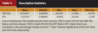
We obtain from Datastream daily prices for the S&P 500 Index and the corresponding ETF (ticker: SPY). The 3-month T-bill rates from January 1954 to April 2010 are from the Federal Reserve Board. We calculate daily returns by the percentage change in daily close prices. Throughout the paper, we use index returns as a proxy for index mutual fund returns.

Table 1 shows the summary statistics. As can be seen, daily returns for the S&P 500 Index and SPY are significantly positive, indicating an upward trend in the stock market. SPY returns have wider swings than the S&P 500 Index returns as evidenced by the larger absolute values for the minimum, maximum, and standard deviation. Returns between the two are highly correlated, with a Pearson correlation coefficient of 0.98, which is not surprising because ETFs are designed to mimic their corresponding indices.

The TOM Effect in the S&P 500 Index Returns and ETF Returns

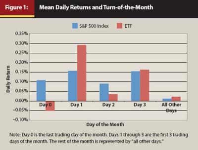
Figure 1 exhibits the mean daily returns across the month. For the S&P 500 Index, the mean daily returns are positive across the days of the month; however, the returns seem to be much higher during the four-day TOM period than during the non-TOM period. For the ETF, the last trading day of the month registers negative average returns but the other three TOM days enjoy positive returns that appear to be much higher than those during the non-TOM days. Thus, Figure 1 shows anecdotal evidence that daily returns are higher during the TOM period than during the non-TOM period.

We divide the sample into two. The first subsample is for the period of no ETF trading. The second subsample is for the period with ETF trading. We conduct a t-test on the mean daily returns across different days of the month.³ Table 2, Panel A shows the results from the sub-period with no ETF trading. As can be seen, the S&P 500 Index daily returns during the four-day TOM window are statistically positive. In contrast, daily returns during the non-TOM period are insignificant from zero. Our results are consistent with the findings in McConnell and Xu (2008). Thus, the four-day TOM window contributes most of the positive returns in the S&P 500 Index, highlighting the fact that investors cannot afford to miss this four-day window.

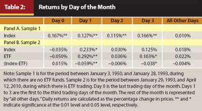
Table 2, Panel B presents the results from the period in which ETF trading is available. Quite different from those in Panel A, for the S&P 500 Index, mean daily returns are significantly positive only on the first trading day and are insignificant for either the other three TOM days or for the non-TOM period. These results are consistent with those in Kunkel, Compton, and Beyer (2003), which found a significantly positive return only on Day 1 of the month for the S&P 500 Index between August 1988 and July 2000. However, these results contrast with those in McConnell and Xu (2008), which shows a significantly positive return on every one of the four TOM days in the CRSP broad market indices between January 1925 and December 2005. Because we use the S&P 500 Index and McConnell and Xu (2008) use the CRSP stock indices, the discrepancy can be attributed to the inclusion of many smaller stocks in the CRSP indices. On the other hand, for the ETF, mean daily returns are significantly positive only on the first trading day and the third trading day of the month. The size of mean daily returns is also larger for the ETF returns than for the S&P 500 Index returns on these two days.

Table 2, Panel B also exhibits the results from a t-test on the daily return difference between the index and SPY. As can be seen, only Day 1 and Day 3 make significant contributions to the dominance of SPY returns over the index fund returns. During other days, ETF returns and the index returns are insignificantly different from each other. Thus, it is during the TOM period that SPY leaps forward over the S&P 500 Index in generating higher returns.

The results in Table 2 reveal two important findings. First, the TOM effect exists in the S&P 500 Index returns and the ETF returns. Second, the TOM effect in the S&P 500 Index returns migrates toward the first day of the month after the introduction of ETF trading. The window is shrinking for investors interested in exploiting the TOM effect in the S&P 500 Index returns.⁴

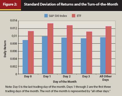
Although returns are higher during the TOM period than during the non-TOM period, is risk also higher during the TOM period than during the non-TOM period? To answer this question, we plot the return standard deviation across different days of the month in Figure 2. For the S&P 500 Index, the standard deviation of daily returns is higher only on the first two days of the month. For SPY, the standard deviation of daily returns appears to be lower during the TOM period than during the non-TOM period. Overall, Figure 2 shows no evidence that risk is significantly higher during the TOM period than during the non-TOM period.

The Returns and Risk of Trading Strategies

Hensel and Ziemba (1996) examine a trading strategy of investing in T-bills during the non-TOM period and switching to investing in the S&P 500 Index funds during the TOM period. They find that this strategy generates an annualized 0.63 percent higher return than the strategy of buying and holding the S&P 500 Index over the period 1928–1993. Similarly, Kunkel and Compton (1998) show that the strategy of investing in the College Retirement Equities Fund (CREF) equity account during the TOM period and switching to investing in a Teachers Insurance and Annuity Association (TIAA) money market fund during the non-TOM period outperforms the index fund buy-and-hold strategy.

We first reexamine the performance of the strategy of investing in T-bills during the non-TOM period and switching to investing in the S&P 500 Index fund during the TOM period, the same strategy examined in Hensel and Ziemba (1996). We label this strategy the T-bill-index-switching strategy. As shown in Panel A of Table 3, this strategy underperforms the index fund buy-and-hold strategy. For example, the monthly return under this strategy is 0.429 percent. In comparison, the index fund buy-and-hold strategy delivers a monthly return of 0.546 percent. Thus, the underperformance is about 1.40 percent on an annual basis. However, the standard deviation of the T-bill-index-switching strategy is lower—about half that of the index fund buy-and-hold strategy. We calculate the Sharpe ratio for the two strategies to compare the reward-risk trade-off. As shown in Panel A, the T-bill-index-switching strategy has a Sharpe ratio of 0.108. In comparison, the index fund buy-and-hold strategy has a Sharpe ratio of 0.079. Therefore, the T-bill-index-switching strategy offers a better reward-risk trade-off than the passive index fund strategy.

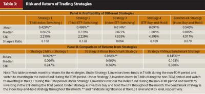
We next investigate the performance of the strategy of investing in T-bills during the non-TOM period and switching to investing in ETFs during the TOM period. We call it the T-bill-ETF-switching strategy. As Table 3, Panel A shows, this strategy generates a higher monthly return than the T-bill-index-switching strategy: 0.498 percent versus 0.429 percent. However, it still underperforms the index fund buy-and-hold strategy: 0.498 percent versus 0.546 percent. In terms of reward-risk trade-off, the strategy of T-bill-ETF-switching has a Sharpe ratio of 0.138, much higher than that for the index fund buy-and-hold strategy, and also higher than that for the strategy of T-bill-index-switching.

We then examine the performance of the strategy of investing in the S&P 500 Index funds during the non-TOM period and switching to investing in ETFs during the TOM period. We call it the index-ETF-switching strategy. As shown in Panel A of Table 3, this strategy outperforms the index fund buy-and-hold strategy by 0.068 percent per month, which corresponds to an annual rate of 0.816 percent. This strategy has a Sharpe ratio of 0.094, which is only higher than that for the index fund buy-and-hold strategy.

Finally, we examine the performance of the ETF buy-and-hold strategy. As shown in Panel A of Table 3, this strategy offers the highest returns. It outperforms the index fund buy-and-hold strategy by 0.145 percent per month, which corresponds to an annual rate of 1.74 percent. This strategy has a Sharpe ratio of 0.109, which is only second to that for the strategy of T-bill-ETF-switching.

In Panel B of Table 3, we conduct a paired t-test to gauge the statistical differences among the performance of various strategies. As can be seen, the strategy of T-bill-index-switching statistically underperforms the strategy of T-bill-ETF-switching. Likewise, the strategy of index fund buy-and-hold statistically underperforms the strategy of index-ETF-switching. In addition, the strategy of ETF buy-and-hold statistically outperforms the index fund buy-and-hold strategy.

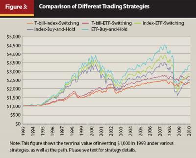
In Figure 3, we illustrate how the value of $1,000 invested in 1993 would fare under the five strategies. We find, consistent with our previous results, that the strategy of index-ETF-switching dominates the strategy of index fund buy-and-hold. Contrasted with the results in Hensel and Ziemba (1996) and Kunkel and Compton (1998), the index-ETF-switching strategy also dominates the strategy of T-bill-index switching and the strategy of T-bill-ETF-switching most of the time—except for the 2007–2009 financial crisis. However, not surprisingly, the strategy of ETF buy-and-hold produces the highest terminal value, which, as indicated in Panel B of Table 2, comes mostly from the first trading day and the third trading day of the month.

Practical Implications for Different Types of Investors

For investors following the passive strategy, the attractiveness of each strategy depends on their tax status, wealth level, and risk aversion. We focus on four types of investors. The first type is the tax-exempted institutional investors. For this type of investor, trading cost for ETFs, about $10–$20 per trade, is minuscule and inconsequential. Thus, the ETF buy-and-hold strategy is superior to the index fund buy-and-hold strategy. Nevertheless, because the strategy of T-bill-ETF-switching has a higher Sharpe ratio than the strategy of investing in ETFs throughout the month, investors still need to choose between the two according to the degree of risk aversion.

Second, for non-tax-exempted institutional investors such as portfolio management firms and high-net-worth individuals with considerable means, trading cost is not a big concern because of the size of the investment. However, there is the factor from the differential tax treatment between long-term capital gains (at 15 percent) and short-term capital gains (at ordinary tax rates that can be as high as 35 percent). Gains under the strategy of ETF buy-and-hold would be considered long-term gains, whereas gains under the strategy of index-ETF-switching are treated as short-term gains. Thus, this type of investor should find the strategy of ETF buy-and-hold most appealing among all the strategies.

The third type of investor is individual investors with taxable retirement accounts. The differential tax treatment would tilt toward the selection of the strategy of ETF buy-and-hold over the strategies involving switching fund types and thus triggering short-term capital gains treatment.

The last type of investor is individual investors with tax-deferred accounts such as 401(k) plans. Many large money management firms offer no-commission ETF trading to their shareholders.⁵ If ETFs are part of the investment-choice set, these investors should prefer the strategy of ETF buy-and-hold over the index fund buy-and-hold strategy. However, as ETFs currently are not part of the investment choice set for most of the 401(k) plans, these investors still have to make a choice between investing in index funds throughout the month or switching from T-bills into index funds during the TOM period. Because trading costs are the same for either strategy, risk aversion will determine which strategy to follow for this type of investor. Nevertheless, this type of investor should demand that commission-free ETFs be added to the investment universe of the 401(k) plans to achieve better returns and reward-risk trade-off.

Conclusion

We examine the returns over the turn-of-the-month period, defined as a four-day window from the last trading day of the previous month to the first three trading days of the current month. We find that returns are significantly higher during the TOM period than during the non-TOM period for the S&P 500 Index and its corresponding ETF. However, the window of the TOM effect seems to shrink in the S&P 500 Index returns after the introduction of ETF trading in recent times.

We investigate the performances of several strategies designed to exploit the TOM effect in returns. Contrasted with early studies such as Hensel and Ziemba (1996) and Kunkel and Compton (1998), the strategy of switching from investing in T-bills during the non-TOM period to investing in index funds during the TOM days underperforms the index fund buy-and-hold strategy. However, the strategy of switching from investing in index funds to investing in the ETF during the TOM days outperforms the index fund buy-and-hold strategy. Overall, the strategy of ETF buy-and-hold offers the highest returns.

For tax-exempted institutional investors and individual investors with large funds, the strategy of ETF buy-and-hold outperforms other alternative strategies. For wealthy investors with taxable accounts, the strategy of ETF buy-and-hold also offers a higher return and a better reward-to-risk ratio. We also highlight the need for 401(k) plans to include ETFs in the investment-choice set for average individual investors to achieve a better reward-risk trade-off for their retirement-investing goals.

Overall, investors need to be aware of the turn-of-the-month effect. With proper considerations for trading costs and taxes, a little market timing on the TOM effect can be return-enhancing.

Endnotes

1. See for example, Ariel (1987); Lakonishok and Smidt (1988); Kunkel, Compton, and Beyer (2003); and McConnell and Xu (2008).
2. As of October 2010, Vanguard offers more than 40 ETFs:
   https://personal.vanguard.com/us/funds/etf.
3. We also divide the sample into four sub- samples: before 1990, 1990–1999, 2000–2007, and 2008–2010. The results remain qualitatively the same. These results are available from the authors upon request.
4. The results from regression analyses show the TOM effect even after controlling for known calendar factors such as the Monday effect, the January effect, the weekend effect, and the financial crisis of 2007–2009. The regression results are available from the authors upon request.
5. With some restrictions, many firms (for example, Fidelity, Vanguard, and TD Ameritrade) offer their investors commission-free ETFs.

References

Ariel, Robert. 1987. “A Monthly Effect in Stock Returns.” Journal of Financial Economics 18: 161–174.

Hensel, Chris R., and William T. Ziemba. 1996. “Investment Results from Exploiting Turn-of-the-Month Effects.” Journal of Portfolio Management 22: 17–23.

Kunkel, Robert A., and William S. Compton. 1998. “A Tax-Free Exploitation of the Turn-of-the-Month Effect: C.R.E.F.” Financial Services Review 7: 11–23.

Kunkel, Robert A., William S. Compton, and Scott Beyer. 2003. “The Turn-of-the-Month Effect Still Lives: The International Evidence.” International Review of Financial Analysis 12: 207–221.

Lakonishok, Josef, and Seymour Smidt. 1998. “Are Seasonal Anomalies Real? A Ninety-Year Perspective.” Review of Financial Studies 1: 403–425.

McConnell, John, and Wei Xu. 2008. “Stock Returns at the Turn of the Month.” Financial Analysts Journal 64: 49–64.

Ogden, Joseph P. 1990. “Turn-of-Month Evaluations of Liquid Profits and Stock Returns: A Common Explanation for the Monthly and January Effects.” Journal of Finance 45: 1259–1272.