Journal of Financial Planning: May 2015
Luke F. Delorme is a research fellow at the American Institute for Economic Research with a focus in retirement studies, investment economics, and personal finance. During his graduate studies, he received The Wall Street Journal award for the top student in the field of finance. He previously worked at the Center for Retirement Research at Boston College, Analysis Group, and State Street Global Markets.
Executive Summary
- Rising equity glide paths during retirement can offer equal or improved financial outcomes compared with static allocations. This study confirms the work by Pfau and Kitces (2014) using a utility model of constant relative risk aversion.
- Increased pension income may encourage retirees to tolerate more risk with retirement savings. Increased risk tolerance entails larger planned withdrawals and/or higher equity allocations.
- As retirees age, pension income (in the form of employer pensions and Social Security) will likely become more important as financial savings dwindle. As a consequence, it is optimal for retirees to increase withdrawals as a percentage of the remaining savings and to increase equity allocation later in retirement. This finding aligns with the benefits of the rising equity glide path.
- Retirement withdrawal amounts have a larger impact on financial outcomes than equity allocations. Retirees should focus first on managing spending before trying to enhance performance through innovative methods of asset allocation.
In their 2014 paper, Pfau and Kitces (2014) sought to determine appropriate equity allocation glide paths for retirees. They found that retirees can reduce risk while sustaining or improving performance by starting retirement with a low allocation to equities and allowing that percentage to increase over time. This is known as the rising equity glide path.
Pfau and Kitces (2014) showed in their research that a portfolio starting at a 30 percent equity allocation and rising to 80 percent will survive in 74 percent of simulations (30-year retirement). A portfolio that maintains a fixed 80 percent allocation to stocks has only a 70 percent chance of success. Perhaps more surprisingly, a portfolio that starts at 80 percent stocks and reduces exposure to 40 percent over the 30-year period has only a 71 percent chance of success. This finding counters the conventional wisdom, which teaches that retirees should shield themselves from risk by reducing equity exposure as they age.
This paper adjusts and extends the Pfau and Kitces (2014) analysis in several ways. First, it recalibrates performance based on a utility model (constant relative risk aversion). This adjustment confirms that rising equity glide paths can offer equal or improved results when compared with static allocations.
Second, it seeks an optimal constant dollar withdrawal percentage in combination with the optimal equity allocation glide path. The analysis finds that withdrawal amounts are more critical to optimal utility outcomes than asset allocation.
Third, it measures performance when pension income is included. Pension and Social Security income act to reduce overall risk exposure. The simulations show that higher pension income, as a ratio to overall wealth, results in an optimal strategy that increases risk exposure through a higher withdrawal and greater exposure to equities. The analysis confirms the value of rising equity glide paths in light of the fact that the ratio of pensions to financial wealth usually increases as retirees age.
The Evolution of Retirement Finance: Safe Withdrawal Rates
If expected returns based on typical stock and bond allocations have historically been 7 percent, it stands to reason that perhaps the safe withdrawal rate could be 7 percent. However, it is far from a guarantee that a balanced portfolio will return 7 percent every year. More likely, there will be significant volatility. In some years returns will be in excess of 7 percent, and in some years returns will be well below 7 percent and possibly negative. This pattern is what led to Bengen’s (1994) seminal work on safe withdrawal rates that established what is now well known as the 4 percent rule.
Bengen’s 4 percent rule suggests that a retiree with $1 million saved could safely withdraw $40,000 per year (inflation-adjusted) and the savings would last at least 30 years. Bengen advocated a portfolio allocation of 50 percent to 75 percent stocks, with the remainder in bonds.
The 4 percent rule is bound by several critical assumptions: it assumes a portfolio accumulation of $1 million; it does not consider how pension income might change the retiree risk profile; and it seeks a constant annual withdrawal amount (inflation-adjusted) and constant equity allocation.
The 4 percent rule has persisted in subsequent research. In 1998, “The Trinity Study” found that a 4 percent initial withdrawal rate, followed by annual inflation-adjusted withdrawals of the same dollar amount, is “extremely unlikely to exhaust any portfolio of stocks and bonds.” In addressing asset allocation, the study finds that “most retirees would likely benefit from allocating at least 50 percent to common stocks” (Cooley, Hubbard, Walz 1998, p. 18). The Trinity Study’s findings on both drawdown percentage and asset allocation confirm the conclusions arrived at in Bengen’s seminal work.
More recently, several studies have sought to determine safe withdrawal rates in today’s economy (Finke, Pfau, Blanchett 2013; Pfau 2011). These studies have largely found that absolutely safe withdrawal rates may actually be below 4 percent (Pfau 2012b). The American Institute for Economic Research’s (AIER) research report on retirement drawdown strategies found that in the 5th percentile of outcomes, a constant dollar drawdown of 3.5 percent is optimal (Delorme 2014). The AIER research suggests that 3.5 percent is the maximum constant drawdown percentage that has been historically safe most of the time.
The common element across the 20 years of research previously discussed is that it seeks an absolutely safe withdrawal rate. The answer is probably somewhere in the vicinity of 3 percent to 4 percent (inflation-adjusted).
Where does this leave households nearing retirement? For a retiree who earned $40,000 a year and saved $1 million, the 4 percent rule bodes well, but how many of these people exist? Recent research from the Center for Retirement Research at Boston College suggests that the typical household aged 55–64 has only $52,600 total in financial assets, 401(k)s, and IRAs (Munnell 2014). As a result, many households nearing retirement may be looking for strategies that maximize income given their limited amount of savings. These strategies will likely involve tweaking portfolio allocations throughout retirement. Equity glide paths are a natural evolution of this desire to optimize retirement income given limited savings.
Equity Glide Path Performance
Financial planners and their clients will always seek innovative asset allocation strategies in an effort to improve financial performance and reduce risk. In response to this desire, Pfau and Kitces (2014) sought to analyze 121 distinct equity glide paths to determine whether simulated performance could be improved compared with static equity allocations. The initial and ending equity allocations range from zero to 100 percent in 10 percentage point increments. The remainder of the portfolio (non-equities) was allocated to intermediate-term government bonds. The research did not intend to find the optimal asset allocation in the realm of modern portfolio theory, but rather to determine whether there is a simple way to reduce risk while maintaining or increasing financial outcomes in retirement.
For each distinct glide path, four measures of retirement performance were measured:
Success rate. This is the likelihood of exhausting assets during a pre-defined retirement window (20, 30, or 40 years) using either a 4 percent or 5 percent initial withdrawal rate with subsequent inflation adjustments. The researchers found that a baseline optimal equity glide path that starts with a 30 percent stock allocation and increases to 80 percent would lead to success in 74 percent of outcomes (30 years at 4 percent withdrawal).
Magnitude of failure. This metric calculates the shortfall in the 5th percentile of outcomes. The magnitude of shortfall is higher when assets are exhausted earlier in retirement. Minimizing the magnitude of failure curtails risk in nearly the worst-case scenario. Pfau and Kitces (2014) found that this measure of performance suggested an optimal rising equity glide path starting at 10 percent and ending at 50 percent for a 4 percent withdrawal.
Median assets remaining at the end of retirement. This measure is the real amount of financial assets remaining at the end of the retirement period in the median outcome of the simulations. This measure suggests a riskier strategy—an optimal allocation that starts at 90 percent equities and rises to 100 percent.
Maximum sustainable withdrawal rate. This is the maximum sustainable withdrawal rate supported at the 10th percentile of outcomes. More similar to the first two measures provided, this measure should appeal to more risk-averse retirees. Using this measure, the researchers found an optimal glide path that starts with 20 percent equities and increases to 40 percent equities, allowing for drawdowns of 3.4 percent annually in the 10th percentile of outcomes.
The various measures show that an array of glide paths could be considered near optimal. If a 74 percent success rate is the best possible scenario, it is reasonable to define “near optimal” as any strategy that results in success 70 percent of the time or better. Under this definition, 92 of the 121 glide paths would be considered near optimal (results are rounded to the nearest whole percent). In other words, the equity glide path has an effect on retirement success, but it is not decisive.
By contrast, when a 5 percent drawdown is used, the optimal equity glide path results in a success rate of only 52 percent. In contrast to the equity allocation, the withdrawal percentage has an outsized impact on retirement success. At any rate, the conclusion is that strategies that use rising equity glide paths instead of fixed or declining equity glide paths often provide equal or better results.
The success rate measure is useful for retirees pursuing a strategy that leads to the lowest chance of exhausting assets. For example, if a retiree has significant financial savings and expects to receive little or no pension income, a strategy that minimizes the chance of failure is paramount. Such a retiree would have extremely high risk aversion. This type of retiree would trade away any chance at upside return if it meant that the chance of failure increased. For this retiree, a reasonable alternative to determining an optimal withdrawal and asset allocation would be to purchase a fairly priced annuity product with a substantial share of the retirement nest egg. Studies have found annuities to be an optimal choice for households with significant financial wealth and high risk aversion (Pfau 2012a and Ameriks, Veres, and Warshawsky 2001).
The model presented in this research offers a fifth measure of retirement outcomes known as the certainty equivalence. Certainty equivalence has regularly been used in the retirement planning literature, but it has rarely (if ever) been used to analyze equity glide paths.
No single metric is perfect for determining the best strategy for retirees, but the certainty equivalence measure may offer a more holistic picture of retirement success. Safe withdrawal rate analyses may be too conservative for many retirees. In a noteworthy study, Finke, Pfau, and Williams (2013) pointed out that “[b]y emphasizing a portfolio’s ability to withstand a 30- or 40-year retirement, we ignore the fact that at age 65 the probability of either spouse being alive by age 95 is only 18 percent … by relying on standard historical or Monte Carlo simulations to determine a safe withdrawal rate, clients may be unduly sacrificing much of their desired lifestyle early in retirement”.
Certainty Equivalence
The certainty equivalence analyzes equity glide paths with a utility model of constant relative risk aversion. The constant relative risk aversion framework is laid out in Blanchett, Kowara, and Chen (2012), Williams and Finke (2011), and Finke et al. (2013). This model calculates the certainty equivalent withdrawal for a stream of retirement income and a given risk aversion parameter (gamma).
A simple example. Take a retirement income stream that provides a 50/50 likelihood of either $30,000 or $40,000 every year as long as a retiree survives. A retiree with a risk aversion parameter (gamma) equal to zero would be indifferent between this pattern and a pattern with guaranteed $35,000 annually. In reality, people tend to have a strong preference toward guaranteed income. Many people would prefer a guaranteed $35,000 annually as opposed to the uncertainty of receiving either $30,000 or $40,000. These people have a positive gamma in the certainty equivalence equation. The certainty equivalent values provided in the results of this paper are given by the following equation.
For any retirement of length N, where ci is the consumption in year i, Pi is the probability of dying in the ith year (joint mortality starting at age 65 is assumed), and γ is the risk aversion parameter:
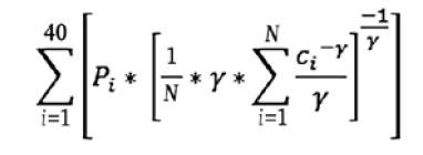
For the purposes of this paper, the baseline gamma is 4. This level is high in order to represent the risk-averse nature of retirees. As noted in Blanchett et al. (2012), results are not very sensitive to the specific gamma chosen. Nonetheless, results using alternative gamma values are noted in several places. Note that there is no bequest motive provided in the certainty equivalence measure, which therefore assumes that retirees seek to maximize spending.
Equity Glide Path Performance as Measured by Certainty Equivalence
This analysis uses a Monte Carlo simulation that selects months at random from January 1926 through November 2014 with replacement to create 1,000 unique return streams (a bootstrapping methodology). Monte Carlo simulation does not account for return momentum and assumes that monthly returns are independently distributed.
In order to most closely imitate the original analysis of Pfau and Kitces (2014), this analysis used stock and bond return assumptions that were less than historical averages. The returns were universally cut so that long-term return averages were similar to those used in Pfau and Kitces. Monthly stock returns, originally produced by the CRSP Deciles 1-10 Index (the market index), received a nominal monthly reduction of 0.27 percent. Monthly bond returns, originally produced by five-year Treasury returns, got a nominal monthly reduction of 0.09 percent. Historical CPI inflation figures were used.
By reducing historical monthly returns, it was possible to produce a series of simulations that had reduced return expectations as compared with history, while maintaining the same volatility and maintaining the historical relationship between stock and bond returns. Summary statistics for the returns are shown in Table 1.
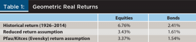
The return assumption significantly influences the optimal glide path. Reduced return assumptions generally lead to more conservative optimal results (lower withdrawal rates and lower equity allocations).
Baseline Results
Certainty equivalences across the simulations were collected for each of the 121 equity glide paths. Strategies were considered near optimal and are outlined in bold in the tables when they fall within 5 percent of the optimal level.
In Table 2, start by looking at the optimal withdrawal and static equity allocation for $1 million in savings with no pension income. The average certainty equivalent suggests an optimal withdrawal of 4 percent with 30 percent allocation to equities. The range of near-optimal strategies encompasses allocations between 20 percent and 80 percent, with withdrawals of either 4 percent or 4.5 percent. This is the first indication that the withdrawal percentage is perhaps more critical than the equity allocation.
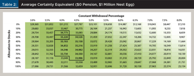
These conservative results are intuitively satisfying because they entail a low-risk retirement strategy. For a household with zero pension income, the possibility of exhausting savings before the end of retirement must be absolutely minimized.
With an increased risk aversion parameter (gamma) of 10, the optimal strategy does not change. With a reduced risk aversion parameter of 1, the optimal strategy increases the withdrawal rate to 4.5 percent and the equity allocation to 50 percent (see Table 6 for a summary of results).
If historical returns are instead used, the optimal strategy increases risk significantly by suggesting a 6 percent withdrawal rate and 80 percent fixed equity allocation. Generally, the larger the difference between assumed stock and bond returns, the more the model will suggest a high equity allocation. Higher assumed returns also endorse higher optimal withdrawals, since increased returns will enable larger withdrawals, especially without any motivation for leaving a bequest. These alternative results highlight the importance of return assumptions, although that is not the focus of this paper.
Next, the results show how equity glide paths can change simulated outcomes. These results are based on a fixed withdrawal amount of 4 percent, as derived from Table 2. The optimal equity glide path on average adjusts the equity share upward from 20 percent to 70 percent over 30 years (see Table 3).
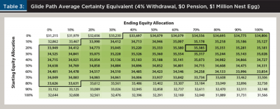
The certainty equivalence increases by a modest 0.4 percent as compared with the static 30 percent equity allocation. In general, equity glide paths that increase over time outperform those strategies that decrease over time. The average certainty equivalence for the 55 increasing equity glide paths ($34,521) is 2.6 percent higher than the average certainty equivalence for 55 declining equity glide paths ($33,655). This difference is not large, but it does confirm that rising equity glide paths improve simulated utility. Note again that there is a wide range of strategies that are within 5 percent of the optimal fixed equity glide path ($35,385 certainty equivalent). This again points out the relative importance of the withdrawal amount.
Results with Pension Income
Pension income, in the form of an employer pension, Social Security, or annuity income, changes household utility. Specifically, guaranteed income reduces the overall retiree risk exposure and allows the optimal strategy with regard to financial assets to increase in riskiness. When the downside risk of a retirement strategy still results in a continual steady stream of certain income, it can encourage retirees to be riskier with non-guaranteed assets (Finke et al. 2013; Milevsky and Huang 2011; Williams and Finke 2011).
Most households have some type of guaranteed pension, commonly in the form Social Security. The following results look at certainty equivalents when a guaranteed pension is included in the income stream. The pension is assumed to be inflation adjusted, similar to Social Security income. Pension income is also assumed to be risk-free.
The results confirm results reported by Finke et al. (2013), Milevsky and Huang (2011), and Williams and Finke (2011). As the pension becomes a larger share of the total financial wealth, it becomes optimal for the equity allocation and withdrawal to become riskier. With an assumption of a $40,000 guaranteed pension and $1 million savings, the optimal strategy withdraws at a rate of 5 percent with an equity allocation of 50 percent (see Table 4; note that the certainty equivalents include the annual pension income).
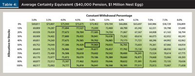
Again, this is intuitively satisfying. Because the worst-case scenario guarantees $40,000 in annual income, households should be more willing to accept some additional risk of exhausting savings. Moreover, as the pension becomes a larger share of the total financial wealth, the range of near-optimal strategies expands. The range of near-optimal withdrawal rates is from 4 percent up to 6.5 percent, and the range of optimal static equity allocation encompasses 10 percent to 100 percent.
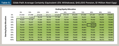
Rising equity glide paths offer another opportunity to improve the simulated certainty equivalence. The optimal glide path for a household with a $40,000 pension starts at 40 percent equities and rises to 80 percent over time (see Table 5). When the pension is included, the range of near-optimal glide paths encompasses almost all of the tested strategies.
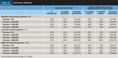
Finally, the analysis looked at summary results across three levels of risk aversion (gamma) and four levels of pensions. As the ratio of pension income to savings rises, savings become a relatively less important part of overall retirement income. The result is that the optimal strategy increases risk by increasing withdrawal percentages and equity allocations.
Another result is that the range of near-optimal outcomes expands as this ratio of pension income to savings rises. At the extreme, consider a household that will receive $80,000 annually from pensions, but has only $100,000 saved for retirement. The savings represent a small share of overall retirement income. The model therefore suggests measurably increasing risk with regard to these savings. At the extreme end of this example, the optimal equity allocation is 100 percent with a 9 percent withdrawal, which is likely riskier than most retirees would realistically consider.
For these reasons, the model may not apply well for households for whom pensions represent the majority of retirement income (Delorme 2015). The risk aversion parameter (gamma) also causes a greater impact when pension income is considered. At low risk aversion levels (gamma = 1) with a $40,000 pension, the optimal withdrawal rate increases to 6 percent with a 70 percent allocation to equities.
Implications for Financial Planners and Clients
The results from this study show that the optimal equity allocations and withdrawals increase as the ratio of pension income to financial wealth increases. The results also show that in many cases, it is considered optimal for retirees to consider rising equity glide paths. These two conclusions are entirely consistent.
As retirees age, they will usually begin to deplete their nest egg (unless withdrawals are very low or returns are very high). When guaranteed pension or Social Security income is constant, this source of income becomes larger relative to the remaining financial savings. The logic follows that it is optimal for the retiree to increase his or her allocation to equities as the pension income becomes a larger share of the retirement income pool. Likewise, if income needs are such that withdrawals must increase as a percentage of the remaining portfolio, the optimal equity allocation should increase. These results and examples highlight that rising equity glide paths are optimal in part because the ratio of pension income to financial assets usually increases as a retiree ages.
Rising equity glide paths may offer an improvement in retirement finance, but a more important factor may actually be the withdrawal rate. A needs versus discretionary income analysis can be very helpful in determining individual utility. By way of example, take a retiree who expects to receive $35,000 annually in Social Security, has $100,000 saved, and places a very high utility on having at least $42,000 a year in retirement. Even at high levels of risk aversion, it seems clear that this retiree may receive high satisfaction from drawing 7 percent annually from their savings. In order to achieve a chance of success, this means that it may be optimal for the retiree to create a risky asset allocation, perhaps 100 percent stocks, or a rising equity glide path that starts with at least 60 percent in stocks.
Now take a retiree with the same pension and savings who determines he needs only $38,000 a year in retirement. This retiree could draw 3 percent annually and maintain a high level of satisfaction. It seems clear that this retiree should draw less, and as a result, can allocate savings much more conservatively. The optimal solution might be to draw 3 percent and allocate only 30 percent to stocks. Should the retiree need a higher withdrawal in the future, an adjustment upward in equity allocation may be prudent.
In summary, when seeking optimal retirement outcomes, financial planners and their clients should first seek to control spending. While higher allocations to equities and rising equity glide paths can improve outcomes, restraining spending will have a greater impact on success or failure.
References
Ameriks, John, Robert Veres, and Mark J. Warshawsky. 2001. “Making Retirement Income Last a Lifetime.” Journal of Financial Planning 14 (12): 60–76.
Bengen, William P. 1994. “Determining Withdrawal Rates Using Historical Data.” Journal of Financial Planning 7 (4): 171–180.
Blanchett, David, Maciej Kowara, and Peng Chen. 2012. “Optimal Withdrawal Strategy for Retirement Income Portfolios.” Retirement Management Journal 2 (3): 7–18.
Cooley, Philip L., Carl M. Hubbard, and Daniel T. Walz. 1998. “Retirement Savings: Choosing a Withdrawal Rate That Is Sustainable.” American Association of Individual Investors Journal 20 (2): 16–21.
Delorme, Luke. 2014. “From Savings to Income: Retirement Drawdown Strategies.” American Institute for Economic Research, Research Studies. www.aier.org/research/savings-income-retirement-drawdown-strategies.
Delorme, Luke. 2015. “Rethinking Retirement Guidelines.” American Institute for Economic Research, Issue Briefs. www.aier.org/research/rethinking-retirement-guidelines.
Finke, Michael, Wade D. Pfau, and David M. Blanchett. 2013. “The 4 Percent Rule Is Not Safe in a Low-Yield World.” Journal of Financial Planning 26 (6): 46–55.
Finke, Michael, Wade D. Pfau, and Duncan Williams. 2012. “Spending Flexibility and Safe Withdrawal Rates.” Journal of Financial Planning 25 (3): 44–51.
Milevsky, Moshe A., and Huaxiong Huang. 2011. “Spending Retirement on Planet Vulcan: The Impact of Longevity Risk on Optimal Withdrawal Rates.” Financial Analysts Journal 67 (2): 45–60.
Munnell, Alicia H. 2014. “401(k)/IRA Holdings in 2013: An Update from the SCF.” Boston College Center for Retirement Research, Briefs. crr.bc.edu/briefs/401kira-holdings-in-2013-an-update-from-the-scf.
Pfau, Wade D. 2011. “Can We Predict the Sustainable Withdrawal Rate for New Retirees?” Journal of Financial Planning 24 (8): 40–47.
Pfau, Wade D. 2012a. “An Efficient Frontier for Retirement Income.” Social Science Research Network, September 24, papers.ssrn.com/abstract=2151259.
Pfau, Wade D. 2012b. “Capital Market Expectations, Asset Allocation, and Safe Withdrawal Rates.” Journal of Financial Planning 25 (1): 36–43.
Pfau, Wade D., and Michael E. Kitces. 2014. “Reducing Retirement Risk with a Rising Equity Glide Path.” Journal of Financial Planning 27 (1): 38–45.
Williams, Duncan, and Michael Finke. 2011. “Determining Optimal Withdrawal Rates: An Economic Approach.” Retirement Management Journal 1 (2): 35–46.
Citation
Delorme, Luke. 2015. “Confirming the Value of Rising Equity Glide Paths: Evidence from a Utility Model.” Journal of Financial Planning 28 (5) 46–52.