Journal of Financial Planning: November 2016
Larry R. Frank, Sr., CFP®, is a registered investment adviser and author. He has an MBA from the University of South Dakota and a bachelor of science cum laude in physics from the University of Minnesota.
Shawn Brayman, MES, is president and CEO of PlanPlus Inc. in Toronto, Canada. He is the 2007 recipient of the Financial Frontiers Award by the Journal of Financial Planning, the 2011 recipient of the Best Paper Award by the Academy of Financial Services, and the recipient of the Best Applied Research award at the 2016 FPA Annual Conference.
Acknowledgement: The authors wish to thank Joe Tomlinson, an actuary and planner, for insightful comments.
Executive Summary
- This paper explored a method that combined actuarial approaches for calculating withdrawals in retirement with Monte Carlo simulations. The model recalculated withdrawals for each scenario within each simulation, with a new simulation beginning for each year based on individual capital remaining and adjusted time horizons using mortality tables.
- The model approach made a direct connection between the various elements making up spending decisions.
- There were important differences between a simulation that used decision rules to shape income and altered initial withdrawal assumptions, and a model that recast each subsequent year in isolation.
- The combination of stochastic simulations and period-adjusting actuarial withdrawal techniques proposed here has been termed Continually Adjusting Stochastic Actuarial Model (CASAM).
One of the most robust areas of research in the field of financial planning is the ongoing search for methods to help clients determine how much they can withdraw from their retirement accounts to optimize their lifestyle while minimizing the chance of ruin due to longevity, portfolio volatility, or poor markets.
This analysis demonstrated the differences between commonly used Monte Carlo simulations that assumed a withdrawal based on a fixed mortality period and initial capital, versus a model that integrated an actuarial withdrawal methodology recasting simulations at the beginning of each year, and for each iteration within each Monte Carlo simulation. The term “Monte Carlo” is used in this analysis to denote stochastic processes in general.
The traditional algorithmic approach and an actuarial approach are based on the same mathematics of determining a payment based on capital, rate of return, and mortality or time horizon. Advisers using algorithmic approaches often understate rates of return or select high mortality assumptions to build in “buffers” for the client. The introduction of Monte Carlo simulations has allowed advisers and software systems to be more precise about the buffers by calculating an initial payment or withdrawal that achieved an acceptable level of failures or successes in the simulated futures.
Rather than try and determine a single “best payment” or even an adaptive payment, this analysis created a model where the actuarial calculation for the payment or withdrawal was rerun every period and in every simulation of possible returns so that it showed how we would make a decision today, five years from now, or 20 years from now, based on revised mortality assumptions and the actual balance of the capital at that time.
The model approach demonstrated that, although a fixed-period simulation had a failure rate at some future age (Frank, Mitchell, and Blanchett 2011), the multiple-period model did not run out of funds unless it was constrained in a manner to cause failure, more in keeping with retiree behavior.
This analysis explained why funds were available at superannuated ages and demonstrated methods that removed the fear of failure (running out of money before life (Milevsky 2016)) to give more control and insight to retirees over the future of their capital. Success or failure did not depend on future markets alone, but also on the retiree’s future spending combined with the rolling effect of aging on time periods used for the simulations.
Bengen (1994) changed the dialogue from a simple algorithmic shortage/surplus to consideration of the probability of failure and estimation of a “sustainable withdrawal rate.” The cost for increased certainty for the client was reduced withdrawals or consumption, and as a result, substantially increased terminal portfolio values should the client die in advance of the assumed time horizon.
Subsequent work, such as Guyton and Klinger (2006) and Klinger (2007) usually using Monte Carlo simulations, explored various conditions or methods by which the initial withdrawal rate could be increased for the client using what have commonly been called decision rule methods.
More recently, work has been done on what is called the actuarial approach. These approaches come almost full circle back to the original algorithmic approach by calculating a payment based on the new actual capital at the beginning of each year and allowing adjustments for revised time horizons and expected future returns.
Waring and Siegel (2015) said: “Spending … should not exceed … a fairly priced level-payment real fixed-term annuity with a term equal to the investor’s consumption horizon” (page 94). Pfau (2015) offered a thorough review of both decision rule and actuarial methodologies.
This analysis extends the current body of knowledge by combining the use of the actuarial methods with Monte Carlo simulations to more accurately model how the withdrawals for the client could evolve over time to replicate aging through the following ways:
- Each year, the time horizon may be revised based on some relationship to mortality;
- Each year, the expected rate of return may be adjusted based on altered capital market assumptions for asset allocation;
- Each year, for each individual scenario within a simulation, the revised capital from the previous year is utilized;
- A revised payment unique to each scenario is calculated based on the previous parameters;
- And, the payment or withdrawal may be further adjusted to generate additional smoothing of income.
A practical manifestation of the difference is that in a simulation, the second-year result is influenced or shaped by the initial first-year conditions and results. These approaches may use decision rules, similar to those first suggested by Guyton and Klinger (2006) for example, to shape future cash flows (essentially a form of modified endowments), but the outcome is to change the solution at the beginning of the simulation or calculation, or chain decisions to the beginning.
In the new model presented in this analysis, each year a unique set of conditions was independent of the preceding conditions because each year was simply recalculated. A traditional model approach would generate the same recommendations between a 60 year old who, after 10 years, had $900,000 left with a balanced portfolio, and a 70 year old with the same capital and portfolio. How either got to age 70 with their capital is irrelevant. What is relevant for both at age 70 is how to spend that capital going forward. Intuitively, it makes sense that the advice would be the same regardless if the client had been with a practitioner for a decade or a day.
The new model, termed Continually Adjusting Stochastic Actuarial Model, or CASAM, provides the advantages of actuarial models that avoid failure while allowing the adviser and client to understand the variability of income that may result from risk of the portfolio or changes in time horizon through the model. The analysis also found that the application of certain smoothing mechanisms could be used to reduce income volatility.
Literature Review
A few areas of prior research were combined in this paper, including: the concept of integrating mortality/longevity to determine the length of distribution periods; the concept that retirees voluntarily adjust their spending as they age or markets fluctuate and are subject to income volatility; the concept that portfolio returns are variable year-to-year and allocations may also change over time; the concept that retirees receive periodic reviews and a model should reflect these; and building a model that incorporates these concepts into one that continually adjusts for all of these variables.
The topic of optimal withdrawal strategies in retirement is one of the most active areas of research and discussion. Stout and Mitchell (2006) first used mortality tables to address the concern of an unknown planning horizon, and Frank, Mitchell, and Blanchett (2012a) developed the first model integrating multiple period simulations based on an annual reference to period life tables to determine the distribution period of each simulation separately. Cotton, Mears, and Cotton (2016) used Kaplan-Meier estimates to “explore the conditional probability of a retiree outliving her savings as age progresses, the relationship of the competing risks of death and ruin as age progresses, and the timing of portfolio failures due to poor market returns” (page 34).
Bernicke (2005) found household expenditures declined as retirees aged, and this decline was voluntary. Blanchett (2014) also suggested that retiree spending tended to decline with age, approximately 1 percent per year, and may increase again at later ages due to medical expenses toward the end of life. Economists have known for decades that changes in economic circumstance result in changes in behavior and spending.
Creating simulations that assume simple inflationary increases in spending during retirement disregard consumption behavior during different economic and market environments. For retired individuals, “autonomous consumption … refers to consumption as part of a long-term plan and as a result of habits and commitments. By being autonomous to income, it is not related to raises, but to a retirement budget constrained by the level of available assets.” (Shambo 2008, page 53).
Steiner (2014) outlined a return to fundamentals with an actuarial approach to calculate the withdrawal amount based on the “risk-free interest rate” and the greater of the retiree’s life expectancy or age 95. Waring and Siegel (2015) expanded on the actuarial approach, or as they termed it, an annually recalculated virtual annuity, or ARVA strategy that could be derived from an annuity payout calculation, repeated each period. Pfau (2015) compared 10 variable spending strategies using a consistent set of portfolio return and fee assumptions using an XYZ formula to calibrate initial spending.
Suarez, Suarez, and Waltz (2015) used a fixed period methodology combined with an n – 1 time horizon (i.e., a 30-year period followed by a 29-year period, etc.). However, there was no reference to mortality tables to adjust the ending age. They also addressed success or failure rates by reframing it as a confidence range.
CASAM does not reference success or failure directly, because the application of actuarial withdrawal with mortality tables always presumes some additional time horizon, even if small in years. This analysis diverged from Waring and Siegel (2015) in that the combination of the two methodologies allows advisers to better understand the possible range of incomes a client may experience, regardless of the assumptions used in the actuarial calculation. This analysis is different, because withdrawal assumptions changed for every year, and every scenario iteration within each simulation changed each year as well. The objective was not to arrive at a single withdrawal assumption, but to illustrate to the client the nature and shape of income in the future and to replicate aging; in other words, to answer the question: what is the estimated range of income and capital by age?
Methodology
Two sets of probability were in play in any projection: probability of the “person,” or mortality table characteristics; and probability of the “portfolio,” or risk and return characteristics of the capital.
Portfolio risk and return characteristics in this analysis came from a globally diversified portfolio developed using MoneyGuidePro. The balanced allocation consisted of 50 percent stocks, 47 percent bonds, and 3 percent cash with a geometric real return of 5.92 percent and standard deviation of 10.24 percent. All results are gross before taxes.
Understanding that portfolio parameters will not remain fixed, defensive and moderate-growth portfolios were tested in addition to the balanced portfolio, as well as different glide paths switching from aggressive to conservative portfolios, or the opposite. Also, because the model calls for annual recalculations, advisers could incorporate different portfolio parameters at any time period interval desired to replicate possible changes he or she may foresee during periodic reviews with clients.
A standard Monte Carlo randomization was used for each set of capital market assumptions with the generation of 1,000 scenarios and 50 periods (ages 60 to 110). The approach was to construct a traditional decumulation simulation using a fixed withdrawal based on a fixed time horizon assumption (for example, 35 years for a 60-year-old client). CASAM used the same return assumptions, but the time horizon was established using mortality tables.
The actuarial calculation of payments is well documented by many authors including Steiner (2014); Waring and Siegel (2015); Pfau (2015) and others, expressed in Excel as:
PMT (rate, nper, pv, fv, type)
Where type determines the beginning-of-period or end-of-period payment. The CASAM algorithm is an end-of-each-period n withdrawal:
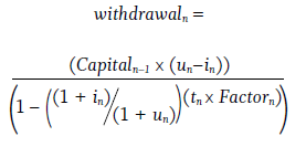
The algorithm was applied individually to each of the 1,000 scenarios. For example, for calculating the Withdrawaln for scenario 101 of 1,000, where n is the year, then
Capitaln – 1 would be the specific capital from scenario 101 from the preceding year; un is the expected return for all scenarios in year n; in is the inflation rate, which is the same for all scenarios in all years (for real returns in = 0); tn is the anticipated mortality or remaining time horizon at year n, which is constant for all scenarios in that particular year n and can be adjusted for mortality variances; and Factorn is the exponential effect adjustment 1 – (1/n), or any other smoothing adjustment, to the payment (Frank, Mitchell, and Blanchett 2012b). In this example, scenario 101 is the 101st iteration of 1,000 iterations.
The term “scenarios” is used here to signify the summation of all iterations
over the number of periods (for example, scenario 101 sums all 101st iterations generated from 50 sets of simulations of 1,000 iterations each between ages 60 to 110, where tn is decreasing between one period to the next from period life tables). This is quite different from one Monte Carlo simulation with only 1,000 iterations that ends at a fixed age.
In traditional simulations, each scenario may be comprised of 30 years, for example, of projected values resulting in 30 sampled values for that single scenario. The aggregated result of many scenarios results in the total simulation result that started at that one given age. For example, for a simulation at age 65, 1,000 iterations would be comprised of 30,000 sampled values (30 years x 1,000 scenarios). For a model approach, this process would be recast at age 61, then again at age 62, etc., resulting in 50 sets (for ages 60 through 110) of 1,000 scenarios of sampled values of ever-shortening time periods.
Comparative results between the single-period simulation and multiple-period CASAM should emerge by inputting any combination of return and standard deviation, real or nominal. Period life tables used would also have comparative results between the two methods. For clients, actual portfolio characteristics should be used instead of trying to apply general research observations to specific people. In other words, one of the purposes of this analysis was to replace the attempt to use general rules of thumb with a modeling approach with which retirees may be able to make better decisions today, while seeing the effect of those decisions on future potential outcomes based on their specific facts and situations.
A variety of approaches to mitigate income volatility were explored in this analysis, including reduced volatility (and return) using different portfolios or glide paths; variations in percentile mortality targets or other factors adjusting the mortality assumption; and floor-and-ceiling assumptions.
Mortality or Time Horizon
Because portfolio withdrawals are most sensitive to the time horizon used, a model should evaluate how life table characteristics change the time function with age, and thus withdrawals with age. Fixed-period simulations and deterministic calculations ignore the influence of mortality on time period calculations. Fixed-period simulations have a single time period over which the calculations are performed. Even actuarial calculations fundamentally rely on a single time horizon assumption for each calculation of the payment amount. However, when one also considers the effect where one moves through the mortality tables as one ages, the time periods are not fixed. An error in cash flow (and resulting portfolio balances) results, because the last period of a fixed-period simulation is only one year long, while those still alive at that later age have more than one year of expected longevity.
Cash flows become non-simulated in fixed-period simulations beyond age 95 (or whatever age is targeted, typically implied by the length of the simulation period); while multiple-period models incorporate those subsequent years for retirees who continue to survive.
The longer the distribution period, the lower the cash flow possible, because of the need to fund more years relative to a shorter distribution period. Therefore, the end years of a fixed-period simulation have ever-growing errors in cash flows relative to a multiple-period model. This also means that models incorporating mortality adjustments encourage spending during the early years when the retiree is more likely to be alive (Blanchett and Blanchett 2008), while also reserving capital for those following older years should they be still alive (Frank, Mitchell, and Blanchett 2012b).
The CASAM model thus calculates the first year’s prudent income for each adjusted simulation period and portfolio balance, while also reserving the portfolio balance for future income needs. A series of solutions result, making up a model that reflects real life. Transitions within the model from year to year account for potential decisions retirees may need to make depending on changing facts and circumstances as they age.
As one ages through the period life tables, the number of expected years to live decreases, and the lifespan variance between dying soon and dying a number of years later increases with age; in other words, the coefficient of variation (Mitchell 2010). This leads to an increased uncertainty of death as one ages. In a practical sense, this increases the volatility of the withdrawal amount. If payments were structured to provide income for 20 years, and a year later instead of 19 years remaining the mortality adjustment remains at 20, the impact is far less compared with that of a life expectancy of four years later in retirement, and after an additional year the mortality adjustment remains at four years. Therefore, a statistical improvement is made to spending and capital balances by adjusting the mortality percentile used to determine the length of distribution periods to compensate for the coefficient of variation present in all the mortality tables at older ages.
Steiner (2014) suggested using the greater of mortality or age 95. Waring and Siegel (2015) stated: “Whatever one’s view on the likelihood of living to extreme old age, it seems prudent to provide for oneself to at least age 105 if male, or 110 if female” (page 99).
The definition of life expectancy is 50 percent of the population outliving the statistical time period. The mortality tables used in this paper were based on the Social Security Administration’s period life tables for 2011. For example, 50 percent of females at age 60 die before age 85. The other 50 percent outlive that approximate 25-year period, with six additional years of life expected beyond age 85. Using life expectancy of 25 years, or to age 85, is 10 years shorter than the 35 years to age 95. Age 95 is a common reference age used in fixed-period simulations, although fewer than 13 percent of 60-year-old females may outlive age 95. The effect of using such an arbitrary “ending” age is to penalize the many (87 percent) who don’t outlive age 95 by restricting their spending from age 60. The CASAM model encourages spending during the years the retiree is most likely to be alive to spend it.
The U.S. Social Security table is a general population table and just one of many choices to model mortality data characteristics—all of which are subsets of the same population measured. Other options include national vital statistics reports from the U.S. Centers for Disease Control and Prevention and the World Health Organization’s life tables. Advisers are encouraged to use life tables that align with the retiree’s population subset characteristics to be more reflective of each retiree’s specific circumstances, health, and country population characteristics.
The challenge with using the 50 percent mortality horizon is that in later ages where life expectancy might be only one or two years, the model aggressively spends down remaining capital. If the client does live the additional years, their capital may be severely depleted and the 50 percent of their funds remaining must now stretch an additional year. A few variants to adjust longevity were tested in this analysis including:
- Setting a minimum mortality, which allowed initial withdrawals to remain unchanged past age 80, but slowed withdrawals later in the model;
- Increasing mortality by a fixed number of years;
- And increasing the mortality percentile by 1 percent per year.
Using the 1 percent increase per annum, the time period for remaining distributions was adjusted to an additional nine years expected beyond age 85. This adjustment required a lower cash flow relative to an unadjusted method for the portfolio value to retain funds for income over the longer period. This effect was discussed in Frank, Mitchell, and Blanchett 2012b. Essentially, the model started with percentiles at the center of the mortality distribution curve and slowly moved the percentile toward the right side of the distribution curve, where fewer of those alive outlive the corresponding life table age.
How Did Simulations Compare to the Model?
In Figure 1, the 75th percentile line (red) and 25th percentile line (orange) show a traditional Monte Carlo simulation (MC #1) with a fixed withdrawal. With no variability in withdrawals, poor returns resulted in a failure, while good returns escalated capital exponentially higher.
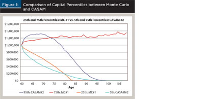
Because CASAM does not adjust income but fundamentally recalculates it, even the most extreme 5th percentile (blue line) and 95th percentile (purple line), representing CASAM #2 usually fell inside the range of the moderate 25th and 75th percentiles of the MC #1 scenario. This illustrates greater predictability of capital outcomes from the CASAM model.
Results
Panel A of Figure 2 shows that the capital from the traditional Monte Carlo (MC) approach (where the income was set to generate a 10 percent failure) had the 5th percentile running out of funds by age 91. Most probability lines escalated exponentially as a result of fixed expected income (constant $40,000 in real dollar terms).
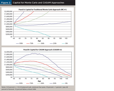
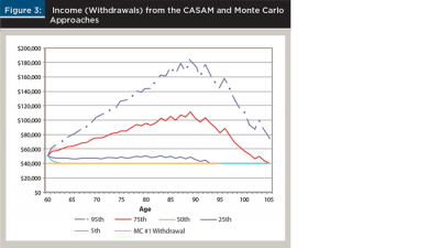
Figure 3 shows the income from the CASAM analysis, which started at about $50,000 and remained stable for the 25th percentile, triggered failures by age 90 for the 5th percentile due to a fixed withdrawal requirement, with income increasing to as much as $180,000 for the 95th percentile.
The objective of the CASAM model is to spend more while the client is likely to be alive, rather than when deceased. A bequest motive may be implemented for retirees who wish to do so. Panel B of Figure 2 illustrates that a bequest is already built into the CASAM model, because the living still require funds for the subsequent years they are expected to live at any given older age. Panel B of Figure 2 shows what that capital may be, given good or bad market trends. The values for the traditional Monte Carlo simulation (Panel A of Figure 2) suggest more capital relative to the CASAM model, however the traditional Monte Carlo simulation ignores future spending adjustments, which would adjust the capital values shown.
If a client is experiencing ongoing bad market returns at the 5th percentile, they will be struggling to make their money last while still funding their expenses. Conversely, a client who is experiencing ongoing great markets at the 95th percentile may spend some amounts above the original expected amounts while allowing the increased accumulation of capital to continue for either increased longevity, estate purposes, or both.
Simple spending simulations typically use failure rates and terminal portfolio values as the measures of success. Pfau (2015) observed that “the frequently used ‘failure rate’ metric should not be applied to variable spending rules” (page 42). This analysis explored a variety of additional metrics to contrast different smoothing strategies including standard deviation of withdrawals, internal rate of return at different percentile outcomes, and mortality-weighted failures and income realized (in other words, a failure at age 100 is less impactful for a 60-year-old client, than a failure at age 80 for a 60-year-old client, because there is less than a 3 percent chance that client will be alive at age 100, but a 70 percent chance that client will outlive age 80).
Table 1 details the statistics from the graphs in Figures 2 and 3. The traditional Monte Carlo scenario used a fixed withdrawal rate where the cash flow was a steady, real $40,000 (replicating the 4 percent rule), which resulted in a 6.8 percent failure rate. The CASAM scenario resulted in a $71,065 withdrawal, but 68 percent of payment was applied, setting the income to $50,338 (68 percent x $71,065), which generated a slightly higher failure rate of 9.9 percent. The 68 percent of calculated income restriction is an example of one possible method to limit spending in order to retain capital for future years.
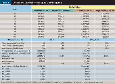
Why is the model in Figure 2, Panel B failing? The failure rate of CASAM was a result of introducing an inflexible floor to spending, essentially forcing the lower percentiles between the Monte Carlo simulation and CASAM to merge on similar results (for example, compare the 5th percentiles in Figure 2). If the spending floor was lowered, the poorer percentiles (5th and higher) improved in CASAM until such time as experiencing no failures once the spending floor was completely removed. Such could be the case where a larger percentage of spending needs comes from pensions, Social Security, and/or immediate annuities. In other words, inflexibility forces portfolio failure in CASAM too, reflecting real life.
The CASAM approach allowed a 20 percent increase in the initial withdrawal for the client, compared to the standard 4 percent rule with a slightly higher failure rate. It resulted in significantly higher mortality-weighted total income and supported income to superannuated ages.
To provide insight into percentiles, Figure 4 pulls out the simulation values showing the first-year spending range percentiles and the 85th year. At age 61, the lower boundary was limited to $40,000, while the 3rd percentile shows $45,586 with CASAM ranging to $60,359 in higher percentiles (97th). At age 85 (the expected longevity at age 60) cash flows are displayed to illustrate how spending variance may occur toward the longer range of spending. Any other age may be similarly evaluated.
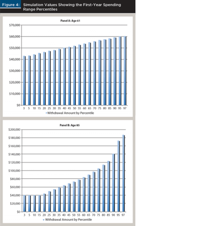
Figure 4 demonstrates that it is possible to model a baseline income and show a possible upside to income if markets permit. Observe that the distribution of percentile results is not a constant by age; for example, the age 85 percentile distribution is different from age 61 in Figure 4. This means that spending should be evaluated each year to determine what is prudent going forward, based on factors known then. The CASAM approach provides a year-by-year evaluation of the range of potential income.
As a person ages beyond age 85, the variance range for income for older ages would narrow as capital narrows until variance is minimal, because there is only one simulation solution given the inputs at that future time for income at that current age, 85. In other words, the wide income variance at age 85 seen in Panel B of Figure 4 would narrow as the Panel A age (looking at one year out) approaches age 85. This is a key insight from CASAM that advisers are not able to observe from Monte Carlo simulations alone.
A method to reduce the volatility of income from a portfolio would be to set the spending from the portfolio at a lower amount and to allow for higher spending only when conditions allowed the portfolio value to grow. This happened in the model automatically when the actuarial method was used to calculate the withdrawal and any reduction factor was applied. The lower income amount may equate to a retiree’s necessary expenses, while the unbounded upper amounts may become the retiree’s new discretionary expenses each year. For detailed trials with a model approach, see Frank and Brayman’s working paper “Certainty of Lifestyle: Contrasting a Simulation over a Fixed Period versus Multiple Period Models” on SSRN at ssrn.com/abstract=2769010.
Conclusions and Practical Application
Here are a few key observations and conclusions:
The CASAM model has a teardrop pattern where ending percentile results tended to concentrate again at the later ages. This refocusing of later-age results may help retirees visualize the consequences of spending levels from earlier ages and the range of incomes they may realize in retirement. There is no need to speculate in the CASAM model on terminal portfolio values that occur using fixed, single-period simulations.
CASAM allows increased spending at earlier years as opposed to approaches that may overly constrain income for the client. The model could also restrain early spending to retain capital for future spending or increased bequests.
When fewer constraints were applied—in other words, flexible spending—the client had a non-zero portfolio balance at all points for the model. Having a minimum spending constraint on a portfolio resulted in running out of funds later during continuously poor scenarios. Having a maximum spending constraint resulted in capital accumulating during continuously good scenarios. Removing these spending constraints resulted in a teardrop pattern, where capital did not run out, nor accumulate, because spending was adjusted based on both the capital and the time remaining.
A higher mortality-weighted total income resulted in all cases using the CASAM model. Retirees would receive money to spend when they were more likely to be alive through the use of applying rolling life table time periods judicially as they aged.
Results showed a higher internal rate of return in all cases using the CASAM model.
In all instances using the CASAM model, there was an automatic bequest at any age. The model always allowed for an extended time horizon. The client required a portfolio balance to fund those future years of income, unless the client spent all the capital.
The CASAM model approach reflected the reality of how people behave by taking multiple reviews as they aged through retirement. Using market-based assets to generate income resulted in portfolio balance variances or volatility.
The final mix of strategies came down to the interaction with the retiree’s risk capacity, defined as an ability to make small adjustments to spending that match income availability at any given point in time.
The result of the simulation was the income solution for that moment in time based on the inputs at that moment. Traditional Monte Carlo simulations ended in a fan-shaped pattern. If there was concern about the length of the simulation period due to health or mortality, adding or subtracting years had a ripple effect on the beginning solution. Advisers performing fixed-period Monte Carlo simulations alone should not infer what the future range of income or capital balances may be due to the errors introduced by differing time frames as the retiree ages. Rolling time periods reflect aging and may encourage spending while the retiree is more likely to be alive.
The CASAM model represented portfolio-based income that was added to pension and/or Social Security. Therefore, if portfolio income represented half of the retirees’ total income, then notionally market effects on a portfolio would only impact half of total income. The planning profession may need to transition thought and practice from a simulation of a single decision and the possible range of outcomes, to a model that serially connects revised decisions based on the remaining period life table time periods a retiree has corresponding to each age, their capital at each point in time, and the range of their limitations of their goal.
It is not suggested here that there is only one way to model portfolio-based income using mortality-based simulations. However, this analysis demonstrated that there are differences between simulations alone and rolling-period, actuarial-based models built upon a series of simulations with important transitions between those simulations that are more reflective of real-life aging and the common practitioner practice of periodic reviews. Hopefully, the concepts outlined here will increase the demand from advisers for this type of model, and solution providers will evolve to meet this demand, because programming capability—which is currently limited to doing one simulation in today’s software, for example Excel—is underutilized.
References
Bengen, William P. 1994. “Determining Withdrawal Rates Using Historical Data.” Journal of Financial Planning 17 (3): 172–180.
Bernicke, Ty. 2005. “Reality Retirement Planning: A New Paradigm for an Old Science.” Journal of Financial Planning 18 (6): 56–61.
Blanchett, David. 2014. “Exploring the Retirement Consumption Puzzle.” Journal of Financial Planning 27 (5): 34–42.
Blanchett, David M., and Brian C. Blanchett. 2008. “Joint Life Expectancy and the Retirement Distribution Period.” Journal of Financial Planning 21 (12): 54–60.
Cotton, Cary., Alex Mears, and Dirk Cotton. 2016. “Competing Risks: Death and Ruin.” Journal of Personal Finance 15 (2): 34–40.
Frank, Larry R., John B. Mitchell, and David M. Blanchett, 2011. “Probability-of-Failure-Based Decision Rules to Manage Sequence Risk in Retirement.” Journal of Financial Planning 24 (11): 44–53.
Frank, Larry R., John B. Mitchell, and David M. Blanchett. 2012a. “An Age-Based, Three-Dimensional Distribution Model Incorporating Sequence and Longevity Risks.” Journal of Financial Planning 25 (3): 52–60.
Frank, Larry R., John B. Mitchell, and David M. Blanchett. 2012b. “Transition through Old Age in a Dynamic Retirement Distribution Model.” Journal of Financial Planning 25 (12): 42–50.
Guyton, Jonathan T., and William J. Klinger. 2006. “Decision Rules and Maximum Initial Withdrawal Rates.” Journal of Financial Planning 19 (3): 48–58.
Klinger, William J. 2007. “Using Decision Rules to Create Retirement Withdrawal Profiles.” Journal of Financial Planning 20 (8): 60–67.
Milevsky, Moshe A. 2016. “It’s Time to Retire Ruin (Probabilities).” Financial Analysts Journal 72 (2): 8–12.
Mitchell, John B. 2010. “A Modified Life Expectancy Approach to Withdrawal Rate Management.” Presented at Academy of Financial Services annual meeting, Denver, Colorado. www.ssrn.com/abstract=1703948.
Pfau, Wade D. 2015. “Making Sense Out of Variable Spending Strategies for Retirees.” Journal of Financial Planning 28 (10): 42–51.
Shambo, James A. 2008. “The Hedonic Pleasure Index: An Enhanced Model for Spending Inflation.” Journal of Financial Planning 21 (11): 44–55.
Steiner, Ken. 2014. “A Better Systematic Withdrawal Strategy—The Actuarial Approach.” Journal of Personal Finance 13 (2): 51–56.
Stout, R. G. and John B. Mitchell. 2006 “Dynamic Retirement Withdrawal Planning.” Financial Services Review (15): 117–131.
Suarez, E. Dante, Antonio Suarez, Daniel T. Waltz. 2015. “The Perfect Withdrawal Amount: A Methodology for Creating Retirement Account Distribution Strategies.” Financial Services Review 24 (4): 331–358.
Waring, M. Barton, and Laurence B. Siegel. 2015. “The Only Spending Rule Article You Will Ever Need.” Financial Analysts Journal 71 (1): 91–107.
Citation
Frank, Larry R., and Shawn Brayman. 2016. “Combining Stochastic Simulations and Actuarial Withdrawals into One Model.” Journal of Financial Planning 29 (11): 44–53.