Journal of Financial Planning: June 2017
Sam Pittman, Ph.D., is head of retail solutions, global client strategy, and research at Russell Investments, where he is responsible for global retail asset allocation and client investment strategies. His research includes multi-period dynamic asset allocation, retirement sustainability, personal funded ratios, income replacement, tax-managed solutions, and equity forecasting
Executive Summary
- A model is created to translate a strategic asset allocation into a product allocation using full active, smart beta, and passive investment options based on an individual client’s aversion to active management underperformance risk.
- The model indicates that as a client’s aversion to excess performance variability increases, they should move from active toward passive products; a suggestion that is likely not surprising, but the spectrum between the extremes will be of interest to advisers.
- Per selected modeling assumptions, advisers may want to consider mixed solutions comprised of all three types of products.
- Further, if an adviser has low confidence in mean-excess-return estimates, this may increase performance variability, which in turn can lead the adviser and client toward lower-cost smart beta and passive solutions, per the model.
The debate to invest actively or passively has engaged the financial industry since the early 1970s, when all equity investors were active investors. The publication of A Random Walk Down Wall Street by Burton Malkiel in 1973, which presented an argument for passive investing understandable to the common investor, helped propel passive investing. In 2014, the amount of wealth invested passively by U.S. investors eclipsed 20 percent.1 This represents a sizable shift in assets and thinking about investing. Moreover, the debate on whether to use passive or active investment strategies now includes a middle ground, smart beta2 strategies, which generally are transparent and rules-based like passive strategies while focused on achieving factor exposures or investment beliefs like active strategies.
Given that the spectrum of multi-asset solutions can range from fully passive3 to fully active4, the question at the forefront is: which asset classes to implement with active, passive, and/or smart beta investment strategies? A commonly held belief is that one should invest passively where active opportunity is considered low, such as highly efficient markets like U.S. large-cap equities, and invest actively where markets are less efficient and opportunity is high, such as emerging markets equities and small-cap equities.
For example, Karabell (2015) suggested focusing active management in asset classes that have more return dispersion among securities. From the reward perspective of active management, this line of reasoning may be justifiable, but it doesn’t include the risk perspective, which could be a fundamental reason investors choose passive versus active investments.
In addition to arguments for selective use of active management, studies have also suggested the sole use of passive management, including Fama and French (2010) and Malkiel (2003). Clients commonly seek passive investments to lower investment expenses. However, if the client believed with certainty that excess performance would cover the investment fees he or she is concerned about, the client may be content paying the fee because (in theory), they’d be better off. But active performance is uncertain.
A solution that addresses where to employ active, passive, and smart beta strategies needs to address both the opportunity for outperformance and the risk of underperformance. This article presents a model that balances a client’s expressed preferences for excess performance from active management and the aversion to risk of underperformance.
Implications of Uncertainty
The idea that performance uncertainty should guide allocation decisions is not new. Barberis (2000) and Kandel and Stambaugh (1996) considered the implications of uncertainty of expected returns on the allocation of total wealth for a constant relative risk averse investor. They showed that parameter uncertainty led to a more conservative allocation of wealth.5
Others, including Ceria and Stubbs (2006) and Garlappi, Uppal, and Wang (2007) formulated a view that investors are averse to ambiguity in expected returns or excess returns, and using robust formulations showed that less weight was allocated to return sources with higher uncertainty. Some could argue from a practical perspective that the amount of active risk included in an investment solution should depend on the investor’s tolerance to performance deviations from the benchmark.
The work presented here more closely follows the ambiguity aversion view, in that the approach below penalizes uncertainty in excess performance. This approach is similar to the work of Kahn and Lemmon (2015), which addressed the use of active, passive, and smart beta strategies in a single asset class. Moreover, the approach presented here addresses uncertainty in the actual expected excess return estimates, in addition to performance uncertainty caused from tracking error.
The model in this article produces a recommendation, by asset class, of how much to invest in active, passive, and smart beta products within a multi-asset portfolio. Although this model addresses aversion to performance uncertainty, higher aversion to performance uncertainty naturally leads to less-expensive investment options, thereby lowering the total portfolio fee. This, in turn, addresses fee sensitivity, but it does so by accounting for the underlying issue—underperformance aversion. After presenting the model, this article demonstrates its use on a balanced asset allocation, and subsequently, how an adviser can apply it.
The Product Allocation Problem
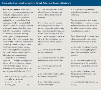
Here it is assumed that the strategic asset allocation is set prior to making product choices for each asset class. Figure 1 illustrates an example of such a decision across three product types: full active, smart beta, and passive for equity and fixed income.
In this example, the client has a strategic allocation of 60 percent equity and 40 percent fixed income. The decision the client and adviser must make is how to allocate the 60 percent equity to full active equity, passive equity, and smart beta equity. Similarly, the client and adviser must decide how to allocate the 40 percent in fixed income.
Figure 1 illustrates these decisions, where in this example for equity, 20 percent is allocated to full active, 10 percent to passive, and 30 percent to smart beta; and in fixed income, 40 percent to smart beta. Although this simple example shows just two broad asset classes, later a balanced portfolio that allocates to 10 asset classes is solved.
Appendix A shows a model that produces decisions on how much active, passive, and smart beta to use in each asset class. The decision is produced by making an explicit trade-off between expected excess performance and the risk of underperforming. The following formula provides a simplified description of the objective in the decision model:
Maximize {expected excess return – fees – risk aversion * variability of excess performance} [1]
However, as noted earlier, many clients do have aversion to performance risk. This aversion is represented in Equation 1 in the third term, where a risk aversion parameter causes the third term of the equation to become smaller (more negative) as the aversion increases. With a high risk aversion, this model guides the decision-maker toward more passive and smart beta investments that have less active performance uncertainty. Of course, a desire for less performance uncertainty reduces fees, because passive and smart beta products tend to be less expensive than full active products. Hence, increasing risk aversion lowers fees.Equation 1 is essentially a utility score that the investor maximizes. Consider that when the risk aversion is zero, the decision is based solely on expected excess return less fees. In this case, if there are positive net-of-fee expected excess-return investment options, the investor will use these vehicles. This represents a client who only cares about expected active performance; not risk.
Implications for Advisers Making Active Decisions
Performance uncertainty due to uncertainty in the mean excess return and the tracking error has implications for advisers making active investment decisions. The excess performance due to tracking error is perhaps less concerning, because over time most advisers expect performance to vary around the expectation; although even modest tracking error can still cause meaningful underperformance over a long horizon, if one is unlucky.
The risk that the actual expected excess return may not match the assumptions used in decision-making is more disconcerting. Consider the disappointment of investing actively based on a prior view of a mean excess return assumption of 1 percent, only to recognize 10 years later that –1 percent would have been a better estimate.
One way to think about the difference in these two risks—mean uncertainty and tracking error—is through a simple analogy. Consider that you bet on coin flipping where you are paid $1 each time heads occurs, and you lose 95 cents each time tails occurs. After 100 flips you expect to make a little money, as this investment has an expectation of 2.5 cents per flip. However, you recognize that you may be unlucky. It’s certainly possible to have more tails than heads in the first 100 flips. The risk of losing money after 100 flips despite a 2.5 percent expected return per flip is similar to the underperformance risk caused by tracking error in active management. Even though you may have a positive net-of-fee alpha expectation, you may get unlucky and lose money.
Consider now in the coin-flipping example that, although you assumed the coin to be fair, it is actually not fair. There is a 45 percent chance of flipping heads, and a 55 percent chance of flipping tails. Although you estimated the expected return to be 2.5 percent per flip, the expected return is –7.25 percent per flip. This type of risk of betting on a negative expected return, thinking it is positive, is similar to risk caused by uncertainty in the estimation of the mean excess return.
Assumptions
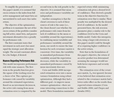
The model in Appendix A is used to show how an asset allocation can be implemented with active, passive, and smart beta products in response to underperformance aversion based on the assumptions in Table 1.
Insights from the Decision Model
The primary interest in solving the product allocation model is to determine how an adviser would change asset class implementation decisions as the client becomes more averse to underperformance. The case of performance variability around the mean (tracking error) is investigated, while a discussion on the impact of mean uncertainty is deferred to later.
To construct solutions for a range of risk aversion levels, the model was first solved with a risk aversion of zero (no aversion to performance uncertainty), and then repeatedly solved for incremental aversion levels. The allocation solution was recorded for analysis.
Figure 2 shows the allocation to active, passive, and smart beta products summed for all asset classes for varied levels of risk aversion. Four fee levels were also indicated, where the total fee was a weighted combination of the underlying asset class product fees based on Table 1.
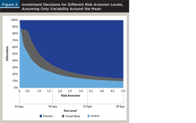
At a risk aversion of zero, the product allocation was 100 percent active, as expected. As the risk aversion increased, the solution moved into both smart beta and passive investments. This happened because as the risk aversion increased, the penalty applied to performance variability increased, incenting the model to decrease performance variability, which of course required higher passive and smart beta allocations.
The risk aversion parameter was scaled so that 5 indicates a high level of aversion, and 0 indicates no risk aversion. At extreme levels of aversion, a near passive allocation was achieved. If the risk aversion was increased high enough, the allocation would move to 100 percent passive, except where a passive option was not included. Similar to classical mean variance optimization where the consideration is the proportion to invest in different asset classes, the risk aversion parameter used here is somewhat abstract. The parameter was varied from 0 to 5 to show how the portfolio changed in response to a higher aversion to active risk. Later, it is explained how an adviser can correlate the solution to a client’s aversion to active risk.
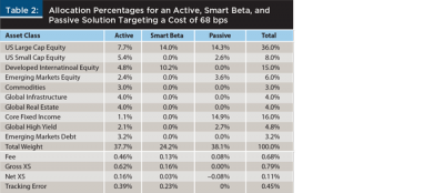
The results in Figure 2 are perhaps most interesting for advisers with clients with moderate aversion to underperformance, where fees range from 40 basis points (bps) to 75 bps. In this range, there was a moderate mixture of active, smart beta, and passive products used. For example, at a fee level of 68 bps, there was approximately 38 percent active, 24 percent smart beta, and 38 percent passive products used. This result is somewhat intuitive, as smart beta is expected to play a larger role when the risk aversion is moderate.
Of course, the relationships shown in Figure 2 were dependent on the capital market assumptions in Table 1, which must come from a careful assessment of skill and factor returns. Although the assumptions are informative for the example here, each adviser would need to evaluate his or her own skill and selective product fees in each asset class to best make use of the model.
A Closer Look at Asset-Class Decisions
Figure 3 shows the percentage of each asset class allocated to an active option for different risk aversion levels. For example, looking at a risk aversion level of 2.5, Figure 3 shows that after infrastructure, which only has an active option, commodities have the highest active allocation, followed by emerging markets debt, global real estate, U.S. small-cap equity, emerging markets equity, developed international equity, global high yield, U.S. large-cap equity, and finally core fixed income. Consistent with Figure 2, as risk aversion increased, the allocation to active management fell in all asset classes where there was a non-active option. However, observe that the model trimmed certain asset classes further than others.
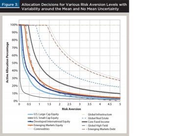
It might seem surprising that asset classes such as U.S. small-cap equity—which is among the asset classes with the highest expected excess return—is not preferred to asset classes with lower expected excess return, such as emerging market debt. Recall from Equation 1 that there were two additional factors that influenced the advice: the risk of not realizing the expected excess return, and the fee. In the model objective, the net-of-fee excess return is being traded off against a penalty for excess return variability. Because the penalty grows as the risk aversion increases, the amount of active management decreases with the risk aversion. But it decreases less so in asset classes that better serve the objective of higher excess return with less risk.
The Impact of Mean Uncertainty
Next, this paper compares how the solution above would differ if the risk of using the incorrect mean excess return was included in the model. Although mean uncertainty exists, it is difficult to measure. Alternatively, tracking error is fairly easy to forecast. Therefore, it was assumed that the mean uncertainty was one-half the tracking error for each product in order to provide a sense of the impact of mean uncertainty on the results.
Figure 4 shows the total active, smart beta, and passive allocations plotted against risk aversion, when the model was solved with and without mean-estimation error. To illustrate, consider a risk aversion of 0.5, resulting in a meaningful allocation to passive, smart beta, and full active management products. When there was no mean-estimation error included, 24 percent of the portfolio was allocated to passive investments. When there was mean-estimation error included, the allocation to passive investments was 49 percent. Indeed, considering that the expected excess return is not known with certainty changes what one should do. However, as the risk aversion increased, the impact of excluding mean uncertainty was muted, as the allocation was moving toward passive in both cases shown.
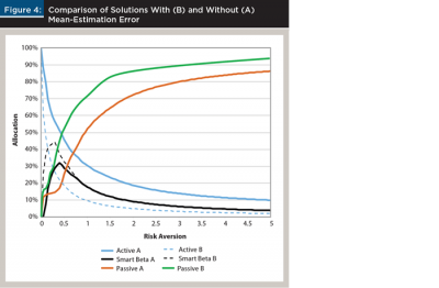
Figures 2 and 3 show that as underperformance aversion increases, more wealth should be allocated to passive and smart beta investments. Figure 4 shows that for the same risk aversion, an investor who considers mean-estimation error would allocate substantially more to passive investments than an investor who did not consider mean-estimation error. Because forward-looking active returns are influenced by both mean-estimation error and variability around the mean, this paper favored a model that included mean-estimation error. However, advisers should recognize the difficulty of constructing confidence intervals for the ex-ante mean excess return. Meanwhile, tracking error is easier to forecast, because it arises naturally in the active management process. For these reasons, the following results show only performance uncertainty related to tracking error.
Trade-Off between Underperformance Risk and Reward
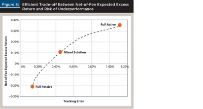
When tailoring a portfolio to meet a client’s aversion to underperformance risk, advisers should seek a product allocation that provides the most excess performance for a given level of underperformance risk. The frontier in Figure 5 provides the most efficient trade-off between net-of-fee expected excess return and the risk of underperformance, which is proxy for tracking error. Indeed, the full active and the full passive solutions were extremes highlighted on the frontier.
Additionally, a solution with a 68 bps fee (a risk aversion of 0.71) is also highlighted in Figure 5 as an example of a mixed active, passive, and smart beta solution that falls between the all active and all passive solutions (see Table 2 for details). This portfolio used sizable allocations to active (38 percent), passive (38 percent), and smart beta (24 percent), putting it in the middle of the range of what’s possible in terms of risk and reward.
Applying the Model to Practice
Advisers and their clients do not have to choose all active or all passive solutions, but advisers should know how to construct efficient portfolios in between these two extremes. To do this, they can suggest a solution that aligns with their client’s unique aversion to underperformance risk. However, just like with absolute risk aversion, clients will not express their aversion to active risk in terms of a risk tolerance parameter value. Moreover, many may express their active risk aversion in terms of total portfolio cost.
Given this, the following practical implementation is suggested for helping advisers choose the optimal portfolio for their individual client:
First, solve the model in Appendix A for varied values of the risk tolerance parameter to obtain an efficient frontier in terms of active return and active risk, just as in Figure 5.
Next, a selection of solutions on this frontier may be chosen. In practice, solutions produced from models are typically adjusted based on sound judgements. It is suggested that advisers do the same here, while using the model as a guide.
For example, a full active portfolio may be used to represent low aversion to underperformance risk, a full passive portfolio may be used to represent high aversion, and a portfolio in between these two may be used to represent moderate risk aversion. These same portfolios can also be used to represent three different fee levels for clients who express their active aversion using fees as constraints. If three portfolios do not provide enough granularity, more portfolios can easily be constructed.
Then, the adviser can map a client to one of the discrete options based on an assessment of the client’s unique active performance aversion or fee specifications.
Practical Insights Gained from the Model
First, a lack of confidence in active manager selection or aversion to underperformance risk should lead to less active management in the portfolio.
Second, regarding the choice of where to invest actively, a careful assessment is necessary. Although it is fairly obvious to invest actively where there is high confidence and high opportunity, the choice between high opportunity with low confidence, versus low opportunity with high confidence is not as obvious. For example, low opportunity in U.S. large-cap equity with reasonably high confidence may be better than high opportunity in emerging markets equity with low confidence.
This exemplifies the key message of this paper: active, passive, and smart beta product allocation decisions should be based on a careful assessment of reward (net of fees) and risk, not solely on fees.
Conclusion
This paper explored how advisers may allocate among active, passive, and smart beta products for their clients, given fee concerns that come about from an assessment of active insights and active risks. A model (Appendix A) was created to translate a strategic allocation to asset classes into a product allocation using full active, smart beta, and passive investment options. The paper then argued that advisers should help clients make these choices based on their assessment of opportunity and two sources of active risk: performance variability around expectations, and performance risk due to lack of confidence in mean estimates.
Using the model to represent these trade-offs, this paper showed that as a client’s aversion to excess performance variability increased, they should move from active products toward passive products. That advice is probably not surprising, but the spectrum between these extremes is rather interesting. Per illustrative modeling assumptions, advisers may want to consider mixed solutions comprised of all three products.
This paper’s model operates on a risk aversion assessment and other parameters to determine a solution. Low confidence in the mean-excess-return estimates increased performance variability, which in turn led the investor toward lower-cost smart beta and passive solutions. Some advisers ignore the estimation risk of their excess-return expectations, which was shown here to have a meaningful influence on the solution.
Higher allocations to passive and smart beta were also induced from high tracking error when there was risk aversion. Expected excess returns and fees also played an important role, as these were traded off against active risk.
Using a model to inform the product allocation decision is important because there are competing interests in the decision, reward, and risk considerations. A model ensures that reward and risk considerations coming from each asset class are not traded off in isolation.
Endnotes
- See the 2016 Investment Company Fact Book, available at icifactbook.org.
- As defined here, smart beta strategies are transparent and rules-based like passive investing, but they focus on achieving factor exposures or investment beliefs, such as value investing. However, they give investors exposure to a factor without the security selection specifics of active stock pickers or the application of factor exposure timing. Moreover, a smart beta strategy can deliver excess exposures to more than one factor. And some product managers may combine factor exposures to accomplish what they believe will achieve excess performance relative to an index (Barber et al. 2015). See Chow, Hsu, Kalesnik, and Little (2011) for a survey of equity smart beta strategies.
- A fully passive strategy is defined as one that seeks cap-weighted benchmark-like performance.
- A fully active strategy is defined as one that includes strategic factor exposures, potentially the timing of factor exposures, and specific security selection.
- The well-known Black-Litterman model (Black and Litterman 1991) is also often used as a Bayesian approach to blend an investor’s views with prior information.
References
Barber, James, Benett Scott, and Evgenia Gvozdeva. 2015. “How to Choose a Strategic Multifactor Equity Portfolio.” The Journal of Index Investing 6 (2): 34–45.
Barberis, Nicholas. 2000. “Investing for the Long Run When Returns are Predictable.” The Journal of Finance 55 (1): 225–264.
Black, Fischer, and Robert B. Litterman. 1991. “Asset Allocation: Combining Investor Views with Market Equilibrium.” The Journal of Fixed Income 1 (2): 7–18.
Ceria, Sebastián, and Robert A. Stubbs. 2006. “Incorporating Estimation Errors into Portfolio Selection: Robust Portfolio Construction.” Journal of Asset Management 7 (2): 109–127.
Chopra, Vijay K., and William T. Ziemba. 1993. “The Effect of Errors in Means, Variances, and Covariances on Optimal Portfolio Choice.” The Journal of Portfolio Management 19 (2): 6–11.
Chow, Tzee-man, Jason Hsu, Vitali Kalesnik, and Bryce Little. 2011. “A Survey of Alternative Equity Index Strategies.” Financial Analysts Journal 67 (5): 37–57.
Fama, Eugene F., and Kenneth R. French. 2010. “Luck Versus Skill in the Cross Section of Mutual Fund Returns.” The Journal of Finance 65 (5): 1,915–1,947.
Garlappi, Lorenzo, Raman Uppal, and Tan Wang. 2007. “Portfolio Selection with Parameter and Model Uncertainty: A Multi-Prior Approach.” The Review of Financial Studies 20 (1): 41–81.
Kahn, Ronald N., and Michael Lemmon. 2015. “Smart Beta: The Owner’s Manual.” The Journal of Portfolio Management 41 (2): 76–83.
Kandel, Shmuel, and Robert F. Stambaugh. 1996. “On the Predictability of Stock Returns: An Asset Allocation Perspective.” Journal of Finance 51 (2): 385–424.
Karabell, Zachary. 2015. “Solving the Active Vs. Passive Investing Debate.” Barrons.com, posted January 26. Available at barrons.com/articles/solving-the-active-vs-passive-investing-debate-1422304950.
Malkiel, Burton G. 2003. “Passive Investment Strategies and Efficient Markets.” European Financial Management 9 (1): 1–10.
Markowitz, Harry. 1952. “Portfolio Selection.” The Journal of Finance 7 (1): 77–91.
Citation
Pittman, Sam. “A Model for Building a Lower-Cost Portfolio Using Active, Passive and Smart Beta Products.” Journal of Financial Planning 30 (6): 40–48.