Journal of Financial Planning: September 2015
Luke Delorme is a research fellow at the American Institute for Economic Research with a focus in retirement studies, investment economics, and personal finance. During his graduate studies, he received The Wall Street Journal award for the top student in the field of finance. He previously worked at the Center for Retirement Research at Boston College, Analysis Group, and State Street Global Markets.
Executive Summary
- Research on retirement spending strategies usually focuses on what is optimal or sustainable. This study selects from the retirement distribution literature in order to frame a strategy based on individual household characteristics and preferences.
- Financial planners and clients can construct a spending strategy foundation based on annual spending flexibility and whether the client is best served by safe or optimized spending.
- Once this foundation is established, several key determinants help inform the spending strategy blueprint, including an appropriate planning horizon and the relative amount of pension and annuity income that the client expects to receive.
- It is important to assess a client’s tolerance for holding equities, bequest motive, and expected portfolio management fees to properly adjust the blueprint
Considerable research on optimal and sustainable retirement spending strategies has been conducted over the last two decades. This paper aims to guide planners and clients toward an appropriate spending strategy based on client preference. The analysis specifically looks at systematic spending strategies—those that employ a pre-defined method of spending. The intent is to review the lessons from existing research and determine which are applicable to different types of clients. By doing so, planners can help clients approaching retirement draft a strategic blueprint for spending from savings.
It is important to remember that research conclusions presented in the literature are derived from assumptions and inputs made by a researcher. The problem is that every household and every individual has specific needs, considerations, and preferences that cannot always be mapped into a simple model. By their nature, models are an abstraction from reality. The result is that researchers come to varied conclusions, pointing to an array of strategies that may be ideal. A sampling of conclusions from previous retirement spending research includes:
- Constant dollar (inflation-adjusted) spending equal to 4 percent of the original balance is the maximum safe amount for a 30-year retirement period (Bengen 1994), based on historical returns for a portfolio that consists of 50 percent stocks and 50 percent bonds.
- Inflation-adjusted spending starting at 5 or 6 percent of the original balance may be safe for shorter retirements and/or higher stock allocations (Cooley, Hubbard, and Walz 1998).
- The 4 percent rule is not safe. Constant dollar spending equal to 3 percent of the original balance may not even be safe because stock and bond returns in the near future will likely be lower than in the past (Finke, Pfau, and Blanchett 2013).
- Retirees with higher-than-average risk tolerance and an annual pension may optimize spending at an annual amount equal to 7 percent of the original portfolio (Finke, Pfau, and Williams 2012). This is because utility-maximizing retirees with pensions should take on greater risk with non-pension assets (Milevsky and Huang 2011).
- Constant dollar spending strategies are far from optimal. Simple alternatives such as using the IRS required minimum distributions are more efficient (Sun and Webb 2012).
- The optimal strategy varies spending over time using updated mortality probabilities (Blanchett, Kowara, and Chen 2012).
Each section of this study looks at a unique aspect of the retirement spending puzzle. The analysis ignores possibilities that could potentially increase retirement income, such as liquidating a house, working longer, or drastically changing the asset allocation. This paper is aimed at households that will rely on savings for regular income in retirement, as opposed to those that will rely primarily on pensions, annuities, or Social Security.
Data and Methodology
Throughout this study, existing research is presented and the findings are confirmed with an original analysis, which uses a variety of methods and definitions that are briefly described here.
Returns: Equity returns are defined by the CRSP Total Market Index, and bond returns are defined by five-year U.S. Treasury notes. Inflation is measured by the Consumer Price Index using monthly historical data from 1926 through 2014.
Baseline assumptions: The baseline simulation looks at a 65-year-old married couple with life expectancy based on the Social Security Administration’s 2010 period life table. A static 50/50 stock/bond allocation is assumed throughout retirement, rebalanced annually, with $0 in pension income and no fees. These assumptions describe very few actual retirees; however, this unrealistic baseline is useful for comparing strategies and existing research. Taxes are not considered in the analysis.
Baseline simulation: The baseline simulation is a bootstrapped Monte Carlo simulation that was run 1,000 times. Months were randomly selected (with replacement) from the universe of months from 1926 through 2014. The stock, bond, and inflation return streams were generated from the selected months. Alternative simulation techniques were tested in the section on return assumptions.
Strategies: Several spending strategies were examined and tested in this study. For certain types of retirees, the appropriate strategy was clear. For example, retirees who place high importance on knowing they can spend the same amount every year should employ a constant dollar strategy, such as that specified by the 4 percent rule. Retirees looking to optimize spending who are willing to employ variable spending strategies have a wider array of potential strategies. The following strategies were compared (an analysis of many other variable spending strategies can be found in a working paper by Pfau (2015)):
Constant dollar: This is the method employed in Bengen’s 4 percent rule. It uses the initial percentage to calculate a constant annual spending amount, which is annually adjusted for inflation.
Constant percentage: This method selects a percentage of savings and spends that percentage of the portfolio each year. When the portfolio changes in value, total spending will change based on the static spending percentage.
Inflation-adjusted percentage: This method selects an initial spending percentage and adjusts the percentage for inflation each year. If first-year spending is 4 percent and inflation is 10 percent, second-year spending will be 4.4 percent of the remaining portfolio (Delorme 2014).
RMD plus: This method uses the percentage from the IRS required minimum distributions, plus or minus a fixed percentage. In retirement years prior to age 70, the percentage is set to 3.5 percent plus or minus the fixed percentage. RMD + 0 percent would be the IRS’s required minimums beginning at age 70 and 3.5 percent prior to age 70.
In this study, it is assumed that households choose not to use annuities to lock in retirement income. Some research shows that it may be optimal for retirees to allocate at least some portion of the retirement portfolio to annuities (Ameriks, Veres, Warshawsky 2001; Pfau 2013), but in practice, the use of annuities remains low for most retirees.
Inflation: All amounts in the analysis were inflation adjusted to today’s dollars based on simulated CPI inflation.
Outcome measurement: Two measures of retirement outcomes were examined: success rate and utility. The success rate estimates how often a strategy exhausts the portfolio during a pre-defined window, often 30 years. The success rate is easy to measure when a constant dollar strategy is considered, but it lacks analytical value when employed in a variable-spending strategy. For instance, if a strategy always draws 6 percent of the remaining portfolio, the portfolio may “succeed” for 30 years by drawing a miniscule level of income during the later years.
The second measure was a utility model of constant relative risk aversion. The constant relative risk aversion framework was laid out in Blanchett et al. (2012) and others (Delorme 2015a; Finke et al. 2013; Williams and Finke 2011).
Consider the following example: assume a retirement income stream that provides a 50/50 likelihood of either $30,000 or $40,000 every year as long as a retiree survives. A retiree with a risk aversion parameter (gamma) equal to zero would not care about the difference between this pattern and a pattern with guaranteed $35,000 annually. Many people would prefer a guaranteed $34,000 annually as opposed to the uncertainty of receiving either $30,000 or $40,000. These people have a positive gamma in the certainty equivalence equation.
The certainty equivalent values provided in the results of this paper are given by the following equation. For any retirement of length N, where ci is the consumption in year i, Pi is the probability of dying in the ith year, and γ is the risk aversion parameter:

For the purposes of this study, the baseline gamma was 4. This high level was used to represent the risk-averse nature of retirees. As noted in Blanchett et al. (2012), results are not very sensitive to the specific gamma chosen.
The Foundation: Spending Variability and Safety
Build the retirement spending blueprint by first laying the foundation for retirement spending. It was assumed in this study that retirees want a structured spending strategy. For retirees who want to engineer a structured spending strategy, financial planners should first answer two questions:
- Does the client prefer safe spending, whereby the portfolio has a minimal likelihood of running out during a pre-determined period of time? Or does the client prefer optimized spending, where there may be a higher likelihood of exhausting the portfolio, but it will be efficiently spent?
- Does the client need to have a steady and constant income over the course of retirement, or is the client comfortable with income flexibility during retirement?
Based on these questions, four foundations for the retirement spending strategy were developed. Each foundation has been featured in the existing literature, but the research does not usually offer an option between these fundamental goals.
Safe and constant: The retiree wants to maximize a safe constant dollar spending rate that seeks the maximum constant dollar amount that will allow the portfolio to last at least a certain length of time. Research that works toward this goal includes Bengen (1994), Cooley et al. (1998), Finke et al. (2013), and Guyton (2004).
Optimal and constant: The retiree seeks optimal constant dollar spending so that the retiree has the same spending amount every year but also the ability to optimize spending based on mathematical probabilities. This client is concerned not only with spending too much but also with spending too little during retirement. Research that works toward this goal include Finke et al. (2012) and Williams and Finke (2011).
Optimal and flexible: The retiree wants optimal flexible spending. Strategies that provide optimal, flexible income are utility maximizing. These are the strategies that work best with economists’ models of utility maximization. Research examples include Blanchett (2013), Blanchett et al. (2012), and Milevsky and Huang (2011).
Safe and flexible: The retiree wants to maximize safe, flexible spending. Flexible spending can allow for higher potential spending than constant dollar strategies while remaining safe. The drawback is the potential that spending falls below what a safe constant dollar pattern might allow. Research examples overlap with optimized flexible research and include Blanchett (2013) and Sun and Webb (2012).
Selecting a Foundation
This paper proposes a system where financial planners ask basic questions in order to determine retiree preference and an appropriate foundation, if it is not obvious. The first question is shown in the top of Figure 1.
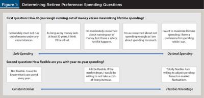
This first question seeks to measure the client’s attitude toward the risk of exhausting assets versus the risk of under spending during retirement. For clients with an absolute aversion to running out of money under any circumstances, it is probably best to guide them toward spending strategies that focus on safety and are aimed to last at least a certain number of years. For clients who prefer enjoying life sooner rather than later and for those who have a robust safety net, an optimized strategy can help maximize lifetime spending and spending efficiency.
The second question (also shown in Figure 1) seeks to measure the retiree’s attitude toward spending variability. If the client needs to know exactly how much to spend every year, financial planners should suggest constant dollar strategies. If the client is somewhat flexible, a strategy such as that proposed in Guyton’s decision rules may be appropriate (Guyton 2004). If retirees are totally flexible, recognizing that market fluctuations may lead to increased or decreased potential spending in any year, a flexible percentage strategy may be most appropriate.
As a sort of tiebreaker, consider a simple analysis of the size of the safety net compared with the total amount of savings. Clients with large relative safety nets (high pensions and annuities compared with savings) may be well served to optimize spending patterns. These strategies tend to entail more uncertainty, but pensions and annuities reduce uncertainty by providing a fixed level of annual income (Milevsky and Huang 2011). With clients who depend more on savings, it may be critical to select a conservative and sustainable constant dollar strategy.
It is important to note here that this analysis has not imposed a strategic spending preference on the client. Some may assume that a client should optimize spending because it is more economically efficient. This analysis does not impose such restrictions. If a client prefers safe, constant dollar spending, that should be the foundation from which the financial planner works.
Existing guidelines and the baseline simulation results are provided in the following section. Next, consider how these results change based on alternative assumptions in the subsequent sections.
Baseline Simulation Results
For clients seeking a safe and constant outcome, Wade Pfau’s website (retirementresearcher.com) offers a retirement dashboard that provides a sustainable spending guideline for a 65-year-old couple retiring today. Safe, constant-dollar spending guidelines for a 65-year-old couple typically range between 3 percent (Finke et al. 2013) to around 4 percent (Bengen 1994; Cooley et al. 1998).
The baseline simulation with a 34-year horizon and a 95 percent success rate finds a safe spending rate of 3.8 percent. This is the baseline amount for retirees with a safe and constant foundation. Alternate options for retirees who are not completely flexible but need higher initial spending should employ a guardrail approach (Guyton 2004; Guyton and Klinger 2006) or a floor-and-ceiling approach (Jaconetti, Kinniry, and DiJoseph 2013). A comparison of these nuanced strategies and others can be found in Pfau’s research (2015).
Retirees seeking optimal constant-dollar spending would be well served to start with an approach advocated by Finke et al. (2012). These researchers optimized the constant-dollar spending amount and equity allocation based on various levels of risk aversion. At a risk aversion parameter of 4 (the baseline measure used in this report), the optimal strategy spends at a 4 percent rate with a 30 percent allocation to equities for a household with a $20,000 Social Security benefit. If the household is more risk tolerant, it may consider spending rates up to 7 percent with equity allocations up to 70 percent.
The baseline analysis shows that the optimal constant-dollar spending is 5.4 percent. This result differs from the findings in Finke et al. (2012) because it uses different returns, includes several more years of positive stock returns, and does not include pension wealth. However, the main finding confirms the existing research, which states that clients who seek to optimize spending should opt for a higher spending rate than those whose primary goal is safety. A baseline of 5.4 percent ($54,000 inflation-adjusted annual spending for a client with $1 million) can serve as the foundation for retirees seeking optimal and constant spending.
A 5.4 percent constant dollar withdrawal results in failure for about 36 percent of baseline 34-year simulations. This is why the spending amount is too high for a retiree looking for a safe spending strategy. However, this spending level fails in only about 16 percent of simulations when life expectancy is considered. In other words, when the probability of success is weighted by mortality probabilities, five in six married couples retiring at age 65 should expect not to exhaust assets using a 5.4 percent constant dollar withdrawal.
Blanchett et al. (2012) measured the relative efficiencies of various spending strategies. They concluded that changing percentage strategies, such as the RMD method, offer significantly improved spending efficiency compared with constant dollar or constant percentage strategies.
Results from this study confirm the results that increasing percentage strategies are more optimal than fixed percentage or constant-dollar strategies for retirees who seek optimality and flexibility (see Figure 2). The utility measure assumes that the retiree is willing to endure potentially lower spending for the opportunity to maximize spending under the more likely scenarios. Utility is maximized from increasing percentage spending strategies, such as the inflation-adjusted percentage strategy starting at 5.6 percent spending, or RMD + 2.7 percent, which starts spending at 6.2 percent. Note that even at safer initial rates as low as 3.5 or 4 percent, the utility of the inflation-adjusted spending strategy is higher than the constant-dollar strategy at its highest utility. This is because the risk of underspending is reduced with inflation-adjusted percentage spending as compared with constant-dollar spending.
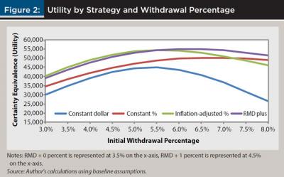
An appropriate approach for retirees seeking safety first but are comfortable with income variability involves using the IRS required minimum distributions as a baseline annual spending guideline (RMD + 0 percent). As an alternative, Blanchett offers a simple spending calculator based on the findings from Blanchett et al. (2012) at www.davidmblanchett.com/tools that can be used to estimate distributions. Blanchett’s calculated spending guidelines are similar to RMD + 0 percent for a 65-year-old couple with a 34-year expected lifespan and 50/50 stock/bond portfolio.
The RMD + 0 percent strategy was tested using spending of 3.5 percent for ages 65 through 69 (before the requirements kick in). The minimum annual spending amount for 1,000 simulated 30-year periods was calculated. The fifth percentile of this minimum annual spending was 2.35 percent of the original portfolio, adjusted for inflation. The RMD strategy also allows for a greater potential upside than the constant-dollar strategy. The median annual spending over each 30-year simulation was calculated, then the median across 1,000 simulations was examined. This “median of medians” was 5.89 percent of the original portfolio, a significant improvement from 3.8 percent fixed spending.
The Retirement Planning Horizon
Once planners have an idea of the desired foundation for the systematic spending strategy, the next element that must be analyzed is an appropriate retirement planning horizon. The 2010 period life table from the Social Security Administration was used to judge the probability of any length of retirement. For clients seeking a safe spending rate, the baseline is a plan that fewer than 5 percent of retirees will outlive. As an alternative, the length of time at which only 1 percent or only 10 percent of retirees would outlive the planning horizon was also considered.
In general, a male retiree should plan to live to about 96 years in order to have a 5 percent or less chance of outliving the plan. A female retiree should plan until age 98. A married couple retiring at age 65 can plan on at least one member of the couple living 34 more years or longer (for a 5 percent or less chance of outliving the planning horizon). Table 1 provides the retirement planning horizon for any household type based on retirement ages from 55 to 80.
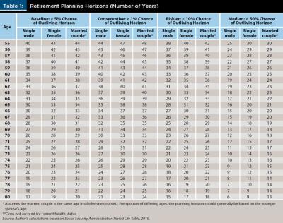
A single male retiring at age 80 has a 95 percent likelihood of living 17 years or less. For a 20-year planning horizon, safe spending rates found in the literature generally increase from about 4 percent to about 5 percent (Cooley et al. 1998). On the other hand, a married couple retiring at 65 may want to plan on a horizon as long as 38 years (for a 1 percent or less chance of outliving the horizon). For this couple, the 4 percent rule may prove to be too dangerous; spending 3.5 percent of the original balance may be more appropriate.
The maximum safe spending rate that results in at least 95 percent simulated success was calculated. For a 34-year planning horizon, the safe spending rate was 3.8 percent (the baseline). For an extended horizon of 40 years, the safe constant-dollar spending rate fell to 3.4 percent. For a shorter horizon of 25 years, the safe rate jumped to 4.6 percent.
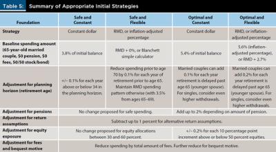
The following planning guidelines can be used to increase or decrease safe and constant spending by 0.1 percentage points for each year more or less than 34 in the planning horizon. For safe and flexible spending, an RMD approach will still dictate the spending percentage for ages 70 and above. During retirement years prior to age 70, spending should be reduced from 3.5 percent by 0.1 percentage points for each year of retirement prior to age 65. For retirement at ages 66 through 69, retirees should exercise caution and maintain 3.5 percent spending during the years before the RMD pattern takes hold.
Clients who choose to optimize spending may find it preferable to spend more early in retirement to maximize lifetime spending. This approach must be balanced by the possibility of living longer than expected.
As the retirement age is delayed, it is optimal to start at a higher level of initial spending (see Figures 3 and 4). The optimal and constant spending percentage increases from 5.4 percent for a married couple retiring at age 65 to 6.0 percent for that couple at age 70. For optimal and constant spenders, married couples could increase spending by 0.1 percentage points for each year that the couple delays retirement beyond age 65 (based on younger spouse’s age).
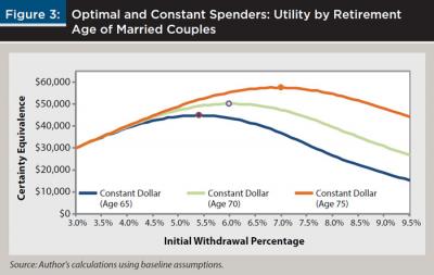
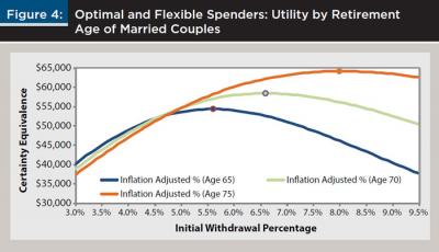
The optimal and flexible strategy is an inflation-adjusted percentage starting at 5.6 percent for a married couple retiring at age 65. The optimal and flexible percentage is 6.6 percent for the married couple retiring at age 70. For optimal and flexible spenders, the initial spending percentage can be increased by 0.2 percentage points for each year a married couple delays retirement beyond age 65. Unmarried retirees, especially men, may choose to further increase spending since they have a shorter potential time horizon than a married couple.
Accounting for Pension Income
To this point, no pension income has been assumed. In practice, many retiree households receive a sizable pension. Some have pensions from corporate or government employers, and nearly everyone has a pension in the form of Social Security. For average retirees, pension income will make up the majority of retirement income (Delorme 2015a; Munnell 2014). Any pension income should be a consideration for utility-maximizing clients.
It has been shown repeatedly in the literature that increased pension income relative to savings should result in riskier strategies for utility-maximizing households, which may entail higher spending or increased equity allocations.
Milevsky and Huang (2011) sought to convince financial planners to advocate flexible spending patterns in order to maximize utility. Their study offers several succinct and thoughtful conclusions, but the one that is applicable here is: “The larger the amount of the pre-existing pension income, the greater the optimal consumption rate and the greater the [portfolio withdrawal rate]” (p. 28). In other words, when pension income is higher, utility is maximized when the initial spending percentage is increased.
The bottom line is that “[a] greater income stream from Social Security, pensions, or annuities increases both the optimal withdrawal rate and allocation toward risky assets” (Finke et al. 2012, p. 49).
In Finke et al. (2012), the optimal constant dollar spending increased from 4 percent to 5 percent for households with $60,000 in pension income as opposed to $20,000. Likewise, Williams and Finke (2011) found that optimal initial spending increases from 5 percent to 6 percent when annual pension income increased from $20,000 to $65,000 (for a 60/40 stock/bond portfolio and gamma equal to 2). This analysis confirms that as the ratio of pension to savings increases, optimal strategies will spend a higher percentage of savings. As this ratio increases, the range of “near optimal” spending percentages widens.
At its most extreme, imagine a household that will receive $50,000 per year from a pension but has only $10,000 saved. If the strategy is to spend 20 percent per year, the household will be able to spend roughly $52,000 for five years and $50,000 thereafter. This income stream is not drastically different from a household that chooses to spend 3 percent per year and may get to spend $50,300 for the length of retirement. Either way, the calculated utility depends mostly on the pension.
At the other end of the extreme, take a household with $1 million in savings and $0 annual pension. The amount this household chooses to spend has a huge effect on utility. If the household spends too much, it may run out of income prior to the end of retirement, a dire circumstance with no safety net.
Table 2 shows the results for optimal spending at various savings-to-pension ratios. A pension of $200,000 may be unrealistic, but a household with savings five times pension income is common (think of a household with $60,000 pension and $300,000 savings). Although the starting spending amounts may be higher than most planners would advise for risk-averse retirees, the pattern of increasing spending at higher relative levels of pension is clear. As the pension becomes more important, the range of near optimal outcomes also widens drastically. Again, this is because the pension is the critical component of retirement income and the structure of the spending strategy becomes less important.
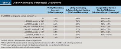
At the low end of the savings-to-pension ratio, the range of near optimal outcomes becomes so wide that there is little formulaic recommendation worth the time of retirees. For these retirees, it may be advisable to throw out systematic spending strategies entirely and instead focus on other priorities (Delorme 2015a).
Finally, clients who seek safe spending strategies will probably not be influenced by the amount of pension. Financial planners can try to encourage those with generous pensions to consider optimal strategies because the safety net is more robust, but retirees focused on safety may not be convinced.
Return Assumptions
The return assumptions used to model retirement income may be the single largest driver of outcomes. Unfortunately, financial planners do not have a crystal ball that predicts future returns. Bengen (1994) simulated historical returns as they happened, assuming that history would repeat itself, or at least that the worst case in history would be no better than the worse possible case in the future.
An alternative assumption would be that future returns will not repeat past returns. Recent research suggests that “the success of the 4 percent rule in the United States may be a historical anomaly” (Finke et al. 2013, p. 46). The compelling evidence for lower safe spending rates are today’s historically low bond yields. Finke and his associates suggested that if bond returns are reduced for just five years, the 4 percent rule may result in failure rates as high as 18 percent. Wade Pfau’s retirement dashboard (retirementresearcher.com) takes into account current equity market valuations and bond yields and suggests a safe initial spending rate below 3 percent, which includes a 0.5 percent annual administrative fee.
Table 3 looks at suggested initial spending based on five different return assumptions. Baseline safe spending can fluctuate from 2.8 to 4.1 percent depending on the return assumption. The advisable action is probably to analyze each retiree’s risk aversion and skew the spending amount appropriately. For financial planners, it may also be important to show the full range of outcomes so that the client can be fully informed of the limitations of any single model.
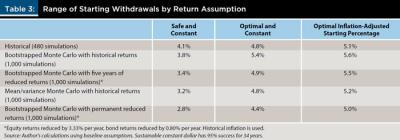
For safe and flexible strategies (not shown in the table), financial planners can potentially reduce the RMD + 0 percent by up to 1 percentage points (the difference between the baseline model and the worst-case model for the safe and constant starting percentage). Alternatively, the Blanchett (2013) simple calculation can be reduced similarly.
Equity Exposure, Bequest Motive, and Fees
Recent research on the optimal asset allocation strategy in retirement suggests that outcomes may be improved with a rising equity glide path, but the findings depend on input assumptions (Kitces and Pfau 2015). Delorme (2015b) found that rising equity glide paths lead to higher utility measures, but the improvement is small compared with static or declining equity glide paths.
This paper is relatively agnostic about asset allocation in retirement. The share of equities in a retirement portfolio may be affected by the amount of pension income, the measure of success, the retirement horizon, and other factors that have been mentioned. It may be difficult to get clients to drastically adjust asset allocations once a decision is embedded.
Although financial planners may hope to guide retirees toward a higher or lower equity allocation, the decision is ultimately made by the client. For this reason, existing research must be adjusted to meet each client’s risk tolerance.
For example, there are circumstances where retirees are not comfortable with an allocation to equities greater than 30 percent. Bengen (1994) found that a 25 percent allocation to equities results in a reduced safe spending rate. Wade Pfau’s website (retirementresearcher.com) offers current sustainable spending rates using three alternative equity allocations based on return assumptions that are lower than historical data.
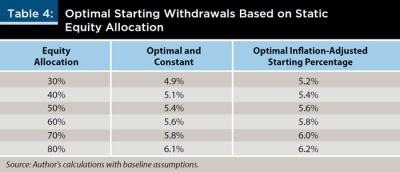
For clients who seek safe spending, this study suggests that no change is needed based on an equity allocation within the range of 30 to 60 percent. The analysis indicates that this range produces a shift of plus or minus only 0.2 percentage points from initial spending. This change is small enough that no spending change is needed based on equity allocation.
For optimal spenders, increased exposure to equities may encourage higher spending. Table 4 looks at the optimized starting percentage under the baseline assumptions for various equity allocations. Generally, an increase of 0.2 percentage points for every additional 10 percent allocated to equities is advised.
Clients may also have strong feelings toward leaving a bequest to their heirs. The math is fairly simple for those with a bequest motive: the lower the spending, the greater the bequest potential. Likewise, the higher the fees, the lower the proposed spending. The analysis to this point unrealistically assumed zero fees. It is reasonable to introduce across-the-board spending reductions equal to the amount of fees regardless of the strategy.
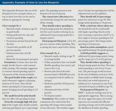
How to Use the Blueprint
Existing research does an excellent job of prescribing retirement spending strategies for specific types of retirees. Most notably, past research has tended to focus on married couples retiring at age 65 with no pension income. The research tends to prescribe either safe or optimal strategies, but not usually a decision between the two.
This study suggests that client preference should drive the spending strategy. A foundation can be engineered that accounts for client preference for either safety or optimization and for either constant dollar spending or variable spending. After these preferences have been revealed, there are systematic ways to adjust the spending amount based on the retirement horizon, amount of pension, return assumptions, equity exposure, bequest motive, and expected fees.
It is hoped that this systematic blueprint will help to provoke client/planner discussions about spending in retirement.
A summary graphic is provided here (see Table 5) that acts as a decision tree to develop an appropriate initial strategy and facilitate client/planner discussions.
Learn More
Interested in retirement spending strategies?
Attend the Journal of Financial Planning/Academy of Financial Services research presentations at the FPA Annual Conference this month in Boston.
Retirement researcher Wade Pfau (one of nine researchers selected to present new research) will discuss the latest on making sense out of variable spending strategies for retirees. View the entire research lineup at FPA-BE.org/academics.
References
Ameriks, John, Robert Veres, and Mark J. Warshawsky. 2001. “Making Retirement Income Last a Lifetime.” Journal of Financial Planning 14 (12): 60–76.
Bengen, William P. 1994. “Determining Withdrawal Rates Using Historical Data.” Journal of Financial Planning 7 (4): 171–180.
Blanchett, David M. 2013. “Simple Formulas to Implement Complex Withdrawal Strategies.” Journal of Financial Planning 26 (9): 40–48.
Blanchett, David, Maciej Kowara, and Peng Chen. 2012. “Optimal Withdrawal Strategy for Retirement Income Portfolios. Retirement Management Journal 2 (3): 7–18.
Cooley, Philip L., Carl M. Hubbard, and Daniel T. Walz. 1998. “Retirement Savings: Choosing a Withdrawal Rate that is Sustainable.” Journal of the American Association of Individual Investors 20 (2): 16–21.
Delorme, Luke F. 2014. “From Savings to Income: Retirement Drawdown Strategies.” American Institute for Economic Research: July 2014 Research Study.
Delorme, Luke F. 2015a. “Rethinking Retirement Guidelines.” American Institute for Economic Research: January 2015 Issue Brief.
Delorme, Luke. 2015b. “Confirming the Value of Rising Equity Glide Paths: Evidence from a Utility Model.” Journal of Financial Planning 28 (5): 46–52.
Finke, Michael, Wade Pfau, and Duncan Williams. 2012. “Spending Flexibility and Safe Withdrawal Rates.” Journal of Financial Planning 25 (3): 44–51.
Finke, Michael, Wade D. Pfau, and David M. Blanchett. 2013. “The 4 Percent Rule Is Not Safe in a Low-Yield World.” Journal of Financial Planning 26 (6): 46–55.
Guyton, Jonathan T. 2004. “Decision Rules and Portfolio Management for Retirees: Is the ‘Safe’ Initial Withdrawal Rate Too Safe?” Journal of Financial Planning 17 (10): 50–58.
Guyton, Jonathan T., and William J. Klinger. 2006. “Decision Rules and Maximum Initial Withdrawal Rates.” Journal of Financial Planning 19 (3), 49–57.
Jaconetti, Colleen M., Francis M. Kinniry Jr., and Michael A. DiJoseph. 2013. “A More Dynamic Approach to Spending for Investors in Retirement.” The Vanguard Group.
Kitces, Michael, and Wade D. Pfau. 2015. “Retirement Risk, Rising Equity Glide Paths, and Valuation-Based Asset Allocation.” Journal of Financial Planning 28 (3): 38–48.
Milevsky, Moshe A., and Huaxiong Huang. 2011. “Spending Retirement on Planet Vulcan: The Impact of Longevity Risk Aversion on Optimal Withdrawal Rates.” Financial Analysts Journal 67 (2): 45–58.
Munnell, Alicia H. 2014. “401(k)/IRA Holdings in 2013: An Update from the SCF.” Boston College Center for Retirement Research Brief.
Pfau, Wade D. 2013. “A Broader Framework for Determining an Efficient Frontier.” Journal of Financial Planning 26 (2): 44–51.
Pfau, Wade D. 2015. “Making Sense Out of Variable Spending Strategies for Retirees.” Social Science Research Network.
Sun, Wei, and Anthony Webb. 2012. “Can Retirees Base Wealth Withdrawals on the IRS’ Required Minimum Distributions?” Boston College Center for Retirement Research Brief.
Williams, Duncan, and Michael Finke. 2011. “Determining Optimal Withdrawal Rates: An Economic Approach.” Retirement Management Journal 1 (2): 35–46.
Citation
Delorme, Luke. 2015. “A Blueprint for Retirement Spending.” Journal of Financial Planning 28 (9): 40–50.
.