Tactical Think Tank: A Fundamental Answer for Tactical Asset Allocation

Journal of Financial Planning: September 2012

Brent R. Brodeski, CPA, CFP^®, CFA, AIFA^®, is the CEO, a principal, and a financial adviser with Savant Capital Management. Brodeski earned a B.S. in finance and economics and an M.B.A., with an emphasis in accounting, from Northern Illinois University. He represented Savant for the fifth year on Barron’s list of the “Top 100 Independent Financial Advisors” in the country. In 2011, Brodeski was named the nation’s 10th “Most Experienced Independent Financial Advisor” by Bloomberg BusinessWeek.

Gina M. Beall, CIMA®, is a senior investment research analyst and member of the Investment Committee with Savant Capital Management. Beall earned a B.S. in business administration with an emphasis in finance from the University of San Diego and an M.B.A. from DePaul University.

Adam W. Larson, CFA, is the investment research team lead and a member of the Investment Committee with Savant Capital Management. Larson earned a B.S. in finance with an emphasis in investments from Northern Illinois University.

Executive Summary

• We were intrigued by the idea of leading RIA firms putting their heads and resources together in a think tank to research one big investment question: might there be ways to predict the market? And if so, could our clients benefit from tactical asset allocation? In other words, was there a silver bullet to time markets after all?
• The Tactical Think Tank LLC (TTT) was formed in 2009 to look at various indicators that may affect a tactical asset allocation strategy. TTT was a group of 10 advisory firms with combined assets under management of about $9 billion. Gobind Daryanani chaired the group.
• After an initial round of research on factors that affect stock market returns, the group split into two research sub-groups: (1) technical and (2) fundamental/strategic.
• This paper addresses our experience with TTT and how we confirmed our belief that there is nothing we know today that can help predict the short-term future—market timing simply does not work. However, we learned that fundamental factors can be used to shape our expectations regarding the intermediate to long term.
• The insights ultimately led us to improve our methodology for calculating long-term, forward-looking expected returns for asset classes. We now use this throughout our financial planning and investment management processes to enhance clients’ wealth.

Many things may come to mind when seeing the name Tactical Think Tank (TTT). At first, the thought of joining such a group seemed counterintuitive to our firm, which is focused primarily on financial planning and long-term strategic asset allocation. However, once we learned about the focus of the group and the membership, we were intrigued by the idea of 10 leading RIA firms putting their heads and resources together to research one big investment question: is it possible to predict the market and benefit from tactical asset allocation? In other words, is there a crystal ball or silver bullet solution for market timing? If so, could we improve our investment process to predict things like the global financial crisis of 2008–2009? As such, TTT was formed in 2009 to look at various indicators that may affect a tactical asset allocation strategy. This was timely, considering that 2008–2009 gave us a great case study to either confirm our suspicions that no crystal ball exists, or provide us a new model to better manage downside risk.

The group of 10 advisory firms had combined assets under management of more than $9 billion and was chaired by Gobind Daryanani.¹ After the group conducted an initial round of research on a range of technical and fundamental factors that affect stock market returns, it was evident that the TTT group should split into two research sub-groups. Half of the firms wanted to focus more on technical factors; the other firms decided to research fundamental/strategic factors. With our company’s focus on long-term asset allocation, we chose to be part of the fundamental/strategic sub-group.

This paper addresses our experience with TTT and how we confirmed our belief that there is nothing we know today that can help predict the short-term future—market timing simply does not work. However, we did learn that fundamental factors can be used to shape our expectations regarding the intermediate to long term. Our participation in TTT led to our development of a decision framework for evaluating different investment strategies and ultimately to improve our methodology for calculating long-term expected returns. We use the long-term, forward-looking returns throughout our financial planning and investment management process to enhance our clients’ wealth.

Sub-Groups and the Factors Studied

At the outset, each TTT firm evaluated either technical or fundamental factors using the following procedure: hypotheses, data tests, observations, and conclusions. The goal was to determine whether any factors provided reliable and consistent signals for making portfolio allocation changes. The 10 firms then split into two groups, fundamental and technical, to further study the most promising factors. Those in the latter group continued to study specific technical signals that showed some evidence in the initial round of research, including: moving averages with Bollinger Bands, moving average convergence/divergence (MACD), leading economic indicator moving averages, mutual fund flows, VIX changes, smart/dumb money sentiment indicator, bull/bear indicator, and equity put/call ratios. In the end, most firms agreed that the “technical” factors did not have enough consistent results to produce confidence in tactical asset allocation. The triggers provided some information about what may happen in markets, but there are inconsistencies and false alerts using solely technical data.

Those in the fundamental camp (including our company, Savant) focused on fundamental factors including dividend yields, price/earnings ratios, yield curves, risk premiums, inflation, long-term trend, and market capitalization. Most did not show predictive power for short-term market returns, but there was evidence that some factors could inform intermediate- and longer-term market returns. In turn, the focus for this sub-group became how to use fundamentals to better predict the market over the longer term. The group developed a framework for categorizing the types of strategic investing as well as expected or forward-looking returns.

Development of a Decision Framework

The basis for the framework can be described using four types of investors with different strategies, which were originally described in Dopfel (2009). The fundamental team, headed by Savant, further classified the investor types and identified the factors each uses to make asset allocation changes (see Table 1).

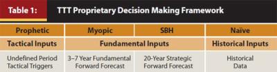
The “naïve” investor sets a long-term strategic investment policy and holds it through all types of regimes (both good and bad economic and financial regimes) and bases decisions on historical returns only. They ignore what is happening today. The “smart but humble” (SBH) investor takes a long-term (20 years or longer) perspective and sets strategic allocations based on that time horizon. The SBH investor recognizes the starting point today and the relevance of fundamental factors, but also recognizes what has happened in the past without relying solely on history. The “myopic” investor also has a forward-looking view, but it is more intermediate-term focused (three–seven years) and makes more significant allocation adjustments along the way. Lastly, the “prophetic” investor ignores the past and future and only focuses on what is happening today, believing they can “time the market” successfully and shift the portfolio in near perfect anticipation of market changes.

The TTT fundamental team is best described with views somewhere between myopic and SBH. The fundamental research provided evidence to support both, but provided the highest degree of support for SBH.

The SBH investor sets a strategic policy that accounts for the uncertainty present in the current regime, while avoiding short-term tactical bets. Being “smart” is to be fully aware of the dynamic economic and financial markets, but being “humble” is to modestly decline to forecast the market in the short term. Academic studies have demonstrated that very few tactical asset allocation strategies outperform long-term strategies. This is particularly the case after trading costs and taxes (Stockton 2010). However, being aware of current circumstances (such as valuations and interest rates) and the direction fundamental factors are likely to move provides information to construct more efficient forward-looking portfolios than naïve buy-and-hold portfolios.

The TTT firms ultimately decided not to formally continue as a group because they concluded there were no reliable and consistent ways to predict and time the market. However, the research conducted in TTT influenced Savant to develop and enhance our formal methodology for setting long-term, forward-looking or expected returns for asset classes. The next several sections discuss Savant’s fundamental research findings in more detail, including how they shape our expected return and asset allocation methodology.

Research on Fundamental Factors: Price/Earnings Ratio

The first topic we address is how stock valuations affect stock market returns. Stock valuations can be measured in different ways, one of which is the price/earnings ratio (P/E). This ratio can indicate whether a stock or stock market’s price is over- or undervalued relative to earnings. Using historical regression analysis, we confirmed that today’s P/E ratio has little correlation with stock returns in the short term, but there is a strong relationship with long-term stock returns.

Our research stemmed from research done by John Y. Campbell and Robert J. Shiller (1998), in which they concluded that conventional valuation ratios—dividend-price and price-smoothed earnings ratios—have special significance when compared with many other statistics that might be used to forecast stock prices. Earnings have been calculated and reported by U.S. corporations for over a hundred years for the express purpose of allowing investors to judge intrinsic value. Corporations have made dividend distribution decisions for just as long, with a sense that dividends should be set in such a way that could reasonably be expected to continue. Campbell and Shiller showed the relationship to be significant over a 10-year period using linear regressions of price changes and total returns on the valuation ratios. While they acknowledge that the analysis that has worked in the past may not work in the future, they do note that the relationships have been examined continually over the last century.

We updated this analysis with data through 2010 and looked at longer subsequent time frames of 20 years. Figure 1 plots the Shiller 10-year P/E ratios (cyclically adjusted)² for U.S. stocks each year since 1881 and subsequent real total returns for various periods. The upper left chart in Figure 1 shows little relationship between the P/E and subsequent one-year returns as evidenced by the flat regression line through all the plotted points. The R2 of 0.052 and correlation of 0.23 are low, indicating a weak relationship. The chart in the upper right shows the correlation for the subsequent five-year periods, which is a slightly stronger relationship with R2 of 0.185 and correlation of 0.43. As the subsequent real total return periods get longer, the relationship gets stronger. For the subsequent 10-year periods, the R2 is 0.308 and correlation is 0.56, and for the subsequent 20-year periods, the R2 is 0.570 and correlation is 0.75.

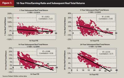
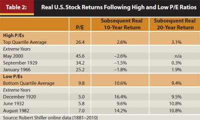
Historically, the relationship between P/E ratios and subsequent returns has been fairly strong over longer periods. History shows that when P/E ratios for U.S. stocks were high relative to the long-term historical average of 17.2, the subsequent returns were below average and even negative. In contrast, when P/E ratios have been low, subsequent stock returns are better than average. Table 2 illustrates this relationship. The average subsequent returns over 10 years and 20 years following periods with P/Es from the top quartile (highest P/Es) are fairly low. Following periods with P/Es from the bottom quartile (lowest P/Es), the subsequent returns were higher than average. The table also shows years with the most extreme historical P/E levels, both high and low. Given this evidence, the current measure of the P/E ratio appears to provide a fairly reliable basis for evaluating long-term return expectations and can be an important factor to consider when calculating long-term expected returns.

Research on Fundamental Factors: Long-Term Trend

Another fundamental factor we studied was what we call long-term trend, influenced by Jeremy J. Siegel’s research (2004 and 2005). Siegel stated that historical evidence provides some clues to future return expectations in which he analyzed the past 200 years of stock, bond, and T-bill data. He showed how remarkably close the cumulative stock returns are to a long-term trend line. The long-term trend line is a straight line, also called a best-fitted regression trend line, which is drawn through the actual cumulative stock returns. Figure 2 shows a similar graph using slightly different data from Robert J. Shiller, which includes 1871 through 2010.

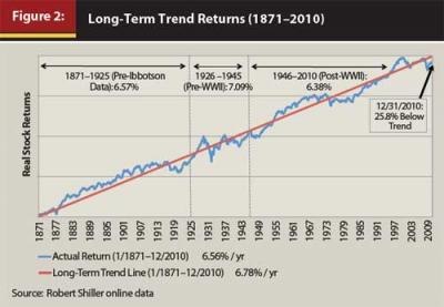
One observation of the calculation Siegel made and that one can make with the updated analysis in Figure 2 is that actual stock returns historically stay very close to the trend line, suggesting mean reversion. The long-term trend line in Figure 2 represents a long-term real stock return of 6.78 percent a year. This trend line can be considered fair market value. In Siegel’s work, he divided historical real returns into major sub-periods to illustrate mean reversion. We do the same with the Shiller data with the full study period having a “real” return of 6.78 percent, and other sub-periods having similar real annualized returns: beginning of good data (pre-Ibbotson), 1871–1925 = 6.57 percent; pre-WWII, 1926–1945 = 7.09 percent; post-WWII, 1946–2010 = 6.38 percent. Across all periods, returns fall between roughly 6 percent and 7 percent, an amazing confirmation of mean reversion.

Applying this concept to expected returns, Savant expects higher returns when actual cumulative returns fall below trend and lower returns when they rise above trend. Building on that concept, we conducted similar regression analysis as we did with valuations and subsequent stock market returns. In this case, we measured the difference of the current market from the long-term trend line and compared that to the subsequent total returns for the stock market over short- and long-term periods. The analysis showed that there is a strong relationship (R2 = 0.62, correlation = 0.79) between the current level of the market relative to the long-term trend and the subsequent long-term (20-year) total return using data from January 1871 through December 1990 (with the subsequent 20-year return period ending December 2010). In other words, when the market level has historically fallen below trend, subsequent returns have been above-trend as the market reverts back toward the long-term average. When we conducted this analysis using shorter subsequent periods, such as one-year returns, there was a weak correlation of only 0.26 and an R2 of 0.068.
A few examples from history further illustrate the findings. In September 1981, actual market prices were 47.1 percent below the long-term trend line, and the subsequent 20-year annualized return was 11.15 percent, an above-trend return. Another example was in July 1967, when the market was 69.0 percent above trend, and the subsequent annualized 20-year return was below trend at 3.97 percent. At the end of 2010, the market was 25.8 percent below trend, suggesting an above-trend return on average over the next 20 years. This is factored into our methodology for calculating forward-looking returns for U.S. stocks.

Research on Fundamental Factors: Dividends

A third area of research was the relationship between dividend yields and future stock market returns. While this paper does not go into detail on the findings there, the conclusion was that the correlation increases with longer periods and that higher dividend yields are associated with higher market returns. It was, however, a weaker correlation than what is evidenced in the price-earnings ratio and trend line comparisons. The issue of stock repurchases makes historical comparisons more challenging. Nevertheless, because dividends are an important component of stock returns over time, we factor dividends into our expected returns methodology for U.S. equity.

Forward-Looking Returns Methodology

While our experience with the TTT did not convince us that investors can successfully time the market, the research on fundamental factors clearly suggests there are things we know and can measure today that can be used to shape our expectations regarding future long-term market returns. The conclusions we drew from our fundamental research and the resulting expected returns methodology have become an important part of our investment process in constructing and managing portfolios.

Our forward-looking return methodology currently spans the following asset classes: global equities (large, small, developed, and emerging), global fixed income (cash, short term, intermediate term, and inflation protected), and alternatives (REITs and commodities).

The forward-looking methodology results in the calculation of expected returns for each asset class. These returns are then used as inputs into the efficient frontier construction. Each asset class has a number of fundamental factors used to calculate expected returns. Below we highlight the methodologies for two of our core asset classes—U.S. equity and U.S. fixed income—which provide the foundation for other equity and fixed income asset class expected returns. Data used are from December 31, 2010, unless otherwise noted.

U.S. Large-Cap Equity

For U.S. large-cap equity, our methodology averages several approaches in order to account for the fact that there is no certainty or exact forecast one can completely rely on. One-third of our expected return is based on valuations where the methodology assumes that the expected return for U.S. large-cap equity is equal to the long-term historical average return adjusted by a valuation factor. The valuation factor is an average calculated by assuming that both the P/E and price-to-book (P/B) ratios will revert to their respective long-term historical averages over a 20-year period. The valuation method calculation shown below suggests U.S. large-cap stocks were slightly overvalued at the time, resulting in a reduction to the historical return.

U.S. Large-Cap Valuation Method³ = Historical U.S. Large-Cap Return (9.9%) + Average Valuation Factor (–1.3%) = 8.6%

The next third of our U.S. large-cap equity methodology is based on a dividend growth expectation. We assume the expected return should be equal to the current dividend yield plus a stock buyback rate, an expected dividend growth rate, and an expected rate of inflation. The components of the dividend growth method resulted in a lower expected return than the historical large-cap return, mainly because of lower yields and expected inflation.

U.S. Large-Cap Dividend Growth Method⁴ = Current Dividend Yield (1.7%) + Repurchase Yield (3.3%) + Dividend Growth Estimate (1.4%) + Long-Term Inflation Estimate (2.4%)⁵ = ((1 + (0.017 + 0.033 + 0.014))*(1.024) – 1) = 9.0%

The final third of our U.S. large-cap equity calculation is based on the long-term trend line methodology we described earlier in this paper. This assumes that cumulative real stock returns will revert to the long-term trend line in 20 years. In other words, the expected return is equal to the annual rate of real return needed for cumulative returns to reach trend in 20 years plus an expected long-term inflation estimate. The components of the long-term trend method resulted in a higher expected return than the historical return, as the actual real returns were 25.8 percent below the long-term real trend line.

U.S. Large-Cap Long-Term Trend Method⁶ = Real Return Required to Get Back to Long-Term Trend Line Return (8.4%) + Long-Term Inflation Estimate (2.4%) = ((1.084*1.024) – 1) = 11.0%

The results from the three methods are averaged and used for the long-term expected return for U.S. large-cap equities: U.S. Large-Cap Equity E(R) = ((8.6% + 9.0% + 11.0%)/3) = 9.5%

U.S. Intermediate-Term Fixed Income

For fixed income, there are two main fundamental factors that go into our expected returns methodology: (1) current yields/interest rates, and (2) expected rate of inflation. We evaluate the level of interest rates and inflation relative to historical norms and the expected direction of each based on current levels.

For example, in the early 1980s, interest rates and inflation were both at record highs. At that time, bond investors could expect reasonably high returns going forward simply because of the high interest payments received from bonds. Also, because bond prices rise when interest rates fall, bond investors could have expected to benefit if interest rates declined from those record high levels. On the other hand, if interest rates and inflation are both low, investors could expect lower returns for bonds going forward. Low interest payments provide lower return from income, and an increase in interest rates would serve to put downward pressure on bond prices.

The methodology we use for U.S. intermediate-term bonds uses the current yield and factors in a long-term credit premium. The later years in the 20-year expected return horizon also factor in an inflation premium. Below is a calculation from December 31, 2010⁷:

First 7-Year Period = Current 7-Year Treasury Yield (2.7%) + Credit Risk Premium (0.2%) = 2.9%

Next 13-Year Period = Long-Term Inflation Estimate (2.4%) + Inflation Premium (3.3%) + Credit Risk Premium (0.2%) = 5.9%

The two period returns are then compounded and annualized over a 20-year period:

U.S. Intermediate-Term Fixed Income E(R) = ((((1 + 0.029)^7)*((1 + 0.059)^13)))^(1/20) – 1 = 4.8%

Other Asset Classes

While we have shown how we apply fundamental factors to U.S. large-cap equities and intermediate-term bonds, it can be important for other asset classes as well. Even with alternative asset classes, simply relying on historical returns can provide a very different viewpoint compared to using facts that we can measure today. Below we highlight recent case studies in commodities and equity real estate (REITs).

The long-term historical return for broad based commodities is about 10 percent.⁸ For purposes of this paper, we assume the sources of return for diversified commodities are: (1) the return from rolling commodities futures/swaps, and (2) the return of the fixed-income collateral. While it is extremely difficult to predict the return from rolling the commodities futures/swaps, our forward-looking return factors in a current expectation for the return of the fixed-income collateral. The fixed-income collateral is typically short-term, high-quality bonds or cash. Given that interest rates are at historic lows today, our expected return for high-quality, short-term fixed income is much lower than history. That expectation results in a long-term expected return for commodities of 7 percent to 8 percent, quite a bit lower than the historical return.

Like commodities, we also found that our expected return for equity REITs is lower than the historical return. Our expected return methodology for equity REITS comprises two main components: current dividend yield and inflation. Both components are lower than what investors have experienced historically. As a result, the long-term expected return for the asset class is currently in the 6 percent to 7 percent range, compared to a historical annualized return of 12.3 percent.⁹

Application of Long-Term Expected Returns

We incorporate expected returns into the work we do for clients in several ways, including: (1) more precise asset allocation and portfolio construction using forward-looking returns, (2) improved guidance for clients to help them determine appropriate asset allocation strategies, and (3) better inputs into financial planning models.

More Precise Asset Allocation. The use of forward-looking returns has a meaningful impact on how we construct and manage portfolios. They are used in traditional mean-variance optimization analysis along with other inputs such as standard deviation and correlation coefficients to help quantify how much to allocate to each asset class. For standard deviation and correlation, we use the historical data (1973–2010) for each asset class as inputs. The standard deviations do not change significantly when measuring long periods, such as 20 years or longer. The correlations have changed over time, as global equity correlations have risen in recent years. However, we do not have reason to believe these will revert back or remain high, so we use a correlation matrix calculated from historical data.

The optimization process is not a perfect science, so we must use additional calculations to construct an efficient frontier that makes sense from both a risk-return perspective and from the perspective of having a globally diversified portfolio. As such, we use a “re-sampling” method to help obtain a smoothed, more-realistic efficient frontier. In addition to re-sampling, we test the sensitivity of the inputs through scenario analysis to evaluate the net impact on the risk-adjusted portfolio returns (change in Sharpe ratio).

Lastly, like most that use mean variance optimization, there are some subjective adjustments to the portfolios instead of just relying on unconstrained optimization—adding a little bit of art to the science. However, we find that these adjustments are not needed as often when we start with better inputs. In this way, the research conducted with TTT helps us take a more scientific approach that is less reliant on the “art” of portfolio construction.

Improved Guidance for Clients to Determine Asset Allocation. Because expected returns change over time, the shape of the efficient frontier changes as well. Thus, it is important to continually evaluate it in conjunction with an investor’s time horizon and risk tolerance (which can also change over time). Figure 3 shows the forward-looking efficient frontier using our expected return methodology during two extreme market periods: March 2000 and March 2009. As a point of reference, we also show the historical risk and return for the same portfolios using data from 1973–2010. The 10 portfolios plotted in the graph start with a 0-100 portfolio (all fixed income) and end with a 100-0 portfolio (all equity).¹⁰

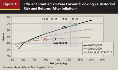
Evaluating the shape and steepness of the efficient frontier provides information that can help an investor determine which portfolio he or she might choose. For example, an investor with a long time horizon might be able to tolerate volatility usually associated with a stock allocation somewhere between 60 percent and 70 percent based on a risk assessment conducted with their adviser. This is identified in Figure 3 as the “sweet spot.” However, most often it is not an exact science for investors when it comes to determining which portfolio within this range to select and when it might be appropriate to consider moving outside that sweet spot. Evaluating the shape of the efficient frontier using forecasting tools (such as Monte Carlo analysis) as well as assessing the investor’s appetite for risk can be very helpful in pinpointing the asset allocation decision.

Looking at the efficient frontier for March 2000, riskier portfolios with higher equity exposure did not offer much additional expected return above the more conservative portfolios. However, they were expected to have much higher volatility. So, an investor who might normally choose between a 60-40 or 70-30 portfolio might have considered a lower volatility 50-50 portfolio (red circle), as taking on more risk would not be expected to produce much more in return. In contrast, the efficient frontier in March 2009 was much steeper. This meant that the expected returns for riskier portfolios were much higher than those of conservative portfolios—the equity risk premium was higher. In this case, an investor who might normally choose between a 60-40 or 70-30 portfolio may want to accept the higher volatility of an 80-20 portfolio (green circle) because the expected premium is high.

Better Inputs into Financial Planning Models. Answering clients’ questions about risk aversion or how much return they need to meet their goals can be very subjective. Thus, having good tools and realistic inputs can provide a better client experience and a higher success rate over time.

Like many advisers, we use expected risk and return calculations in our financial planning process to run Monte Carlo analysis. This analysis provides success probabilities of different scenarios by calculating thousands of iterations over the desired timeframe. Table 3 is an illustration of how the efficient frontier data can be applied to Monte Carlo analysis (using the same periods of 2000 and 2009 from Figure 3—two extreme periods where expected returns varied widely). The assumptions used in the Monte Carlo analysis for Table 3 are $1 million initial investment, 25-year time horizon (typical horizon for a 65-year-old with a life expectancy of 90 years), 5.5 percent (of initial value) withdrawals, expected inflation of 3 percent in 2000 and 2 percent in 2009, and fees of 1.0 percent.

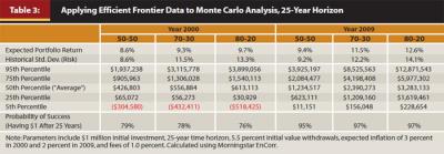
In the year 2000, when fundamental factors suggested that equities were historically overvalued, an investor’s expected outcomes were very similar whether they chose a 50-50 or an 80-20 portfolio. The ending “average” values (50th percentile) were relatively similar for both portfolios ($426,803 and $613,113, respectively). The investor would not expect much more benefit by increasing risk (volatility) with an 80-20 portfolio. The probability of success (having at least $1 left after 25 years) actually decreases with the more aggressive portfolio.

In contrast, fundamental factors in 2009 suggested that equities were undervalued while bonds were expensive. The range of expected ending wealth outcomes varied significantly between the 50-50 and 80-20 portfolios. The difference in the expected value at 25 years for a 50-50 portfolio was $1,234,517 versus $3,283,133 for an 80-20 portfolio, a significant increase. In addition, the upside potential (95th percentile) for the 80-20 portfolio is significantly higher. The downside (5th percentile) is not that different between the two portfolios, but the probability of success (having at least $1 left after 25 years) increases with the more aggressive 80-20 portfolio. The analysis shows that in 2009, the additional expected wealth for the 80-20 portfolio is probably worth the additional volatility.

Reviewing the efficient frontier at different points in time can help shape client expectations and actions. It allows us to provide clients with more realistic expectations while other types of forecasting that rely only on historical returns, simple averages, or straight-line return assumptions might provide overly optimistic or pessimistic outcomes.

Conclusion

As global markets change and evolve, financial planners need to continually revisit how they view investment management and planning. Savant’s participation in the TTT group allowed us to collaborate with some of the top RIA firms in the country to further our thinking as it relates to structuring portfolios and evaluating asset classes. TTT confirmed our belief that there is nothing we know today that can help predict the short-term future—market timing still does not work.

We did, however, find that incorporating a forward-looking returns framework based on measurable fundamental data improves the quality of our advice. TTT participation led us to develop a decision framework to evaluate different investment strategies and ultimately to enhance our methodology for calculating long-term expected returns for asset classes. This moved us toward our ultimate goal of better protecting and growing our clients’ assets in order to help them reach their goals.

Endnotes

1. Gobind Daryanani developed the Intelligent Rebalancer (iRebal) software, which is used by advisers for rebalancing, cash management, and tax harvesting, and has written books and papers on rebalancing.
2. The price-earnings ratios (P/E) used in the analysis are the 10-year smoothed P/E ratios as calculated by Robert Shiller (also known as the cyclically adjusted P/E ratio). www.econ.yale.edu.
3. U.S. Large-Cap Equity Valuation Method: historical U.S. large-cap return = S&P 500 Index total return annualized from 1926–2010 (9.9 percent). P/E ratio = percentage differential between the Shiller 10-year normalized P/E ratio (22.5) and long-term average (16.4) of 37.5 percent annualized over 20 years for a value of 1.6 percent. Price/book ratio = percentage differential between the annual Fama-French P/B ratio adjusted for S&P 500 market return since annual mid-year calculation (2.0) and the long-term average (1.6) of 21.7 percent annualized over 20 years for a value of 0.99 percent. Average valuation factor = (1.6 + 1.0)/2 = 1.3. The 1.3 is a reduction to the historical return based on valuations. Morningstar EnCorr. www.econ.yale.edu. http://mba.tuck.dartmouth.edu..
4. U.S. Large-Cap Dividend Growth Method: current dividend yield = S&P 500 current yield (1.7 percent). Repurchase yield = five-year average of stock buyback levels for S&P 500 calculated as the total stock buybacks divided by the total market value (3.3 percent). Dividend growth estimate calculates the long-term average growth rate (since 1977) in the annual dividend yield; dividends paid divided by S&P 500 Index price (1.4 percent). www.standardandpoors.com.
5. Long-Term Inflation Estimate. Expected inflation is based on an “unbiased” forecast calculated as the current spread between 20-year nominal Treasuries (4.1 percent) and 20-year TIPS (1.6 percent). Subjective adjustment was made using data from the 30-year “unbiased” spread and the “Survey of Professional Forecasters” published by the Federal Reserve Bank of Philadelphia for the 2.4 percent estimate. www.federalreserve.gov.
6. Long-Term Trend Method: historical real value = annualized return of the S&P 500 using historical real returns (6.6 percent). Trend line value = annualized regression of monthly real total returns (0.005480) (6.8 percent). Return required = ending index values calculated for the historical and trend line using monthly returns to determine the differential of being under or over the trend line (–25.8 percent). Next calculation is to determine the required annualized real return to bring the actual real value back to the trend line value over a 20-year period by projecting out the regression index (8.4 percent). Morningstar EnCorr. www.econ.yale.edu.
7. U.S. Intermediate-Term Fixed-Income Method: intermediate risk-free rate = U.S. 7-year Treasury yield (2.7 percent). Credit risk premium = difference between the Barclays U.S. Intermediate-Term Government/Credit Index return (7.8 percent) and the Barclays U.S. Intermediate-Term Government Index return (7.6 percent), equals 0.2 percent. Inflation premium = difference between the long-term average inflation rate (4.4 percent) and the long-term average return of the Barclays U.S. Intermediate-Term Government Index (7.7 percent), equals 3.3 percent. Morningstar EnCorr. www.federalreserve.gov.
8. The historical return for commodities is an equal-weighted blend of the following index returns: S&P GSCI Commodity Index and GRCI Commodity Index (1973–1990), DJ UBS Commodity Index (added in 1991), and Reuters/Jeffries CRB Index (added in 1994). Morningstar EnCorr.
9. FTSE NAREIT Equity REIT Index. Morningstar EnCorr (1973–2010).
10. Portfolios for Savant are composed of the following indices to represent each asset class: Stocks: S&P 500 Index, Fama-French Large Value Index, CRSP Deciles 6-10 Index, Fama-French Small Value Index, MSCI EAFE Index, MSCI EAFE Value Index, Dimensional Int’l Small Cap Index, Dimensional Int’l Small Value Index, MSCI Emerging Markets Index. Bonds: BarCap U.S. Government/Credit Intermediate Index, BofAML U.S. Treasuries Inflation Linked Index, BarCap Global Aggregate Ex U.S. Index. REITs: FTSE NAREIT Equity REIT Index. Commodities: see endnote 8. Real expected returns and volatility (standard deviation) for Savant’s portfolios in 2000 and 2009 were calculated using our forward-looking return methodology for each asset class shown in this endnote.

References

Arnott, Robert D., and Peter L. Bernstein. 2002. “What Risk Premium is Normal?” Financial Analysts Journal (March/April).

Dopfel, Fred. 2009. “The New Policy Portfolio.” Barclays Global Investors, Investment Insights 3, 2.

Shiller, Robert J., and John Y. Campbell. 1998. “Valuation Ratios and the Long-Run Stock Market Outlook.” Journal of Portfolio Management (Winter).

Shiller, Robert J., and John Y. Campbell. 2001. “Valuation Ratios and the Long-Run Stock Market Outlook: An Update.” Cowles Foundation Discussion Paper No. 1295.

Siegel, Jeremy J. 2004. “The Long-Run Equity Risk Premium.” CFA Institute Conference Proceedings.

Siegel, Jeremy J. 2005. “Perspectives on the Equity Risk Premium.” CFA Institute.

Stockton, Kimberly A., and Analtoly Shtekhman. 2010. “A Primer on Tactical Asset Allocation Strategy Evaluation.” The Vanguard Group (August).