Journal of Financial Planning; May 2014
James L. Olsen, CFP®, CFA, is the chief market strategist at First Niagara Private Client Services in Plymouth Meeting, Pennsylvania, where he is responsible for managing and advancing individual client investment portfolios, and where he participates in the firm’s trust investment committee. He leads the firm’s committee that determines tactical asset allocation decisions and conducts new manager searches.
Executive Summary
- This paper examines the impact that the Federal Reserve’s quantitative easing programs have had on equity market prices.
- An estimation of the value of the S&P 500 Index was made on a quarter-end basis assuming that no quantitative easing program had been in place. The estimated value of the index was derived through fundamental valuation techniques using a predicted value for the risk-free rate of return. A comparison of the actual S&P 500 Index was made to the estimated value of the index to measure the valuation differences.
- The study shows that both the first round of quantitative easing (QE1) and the second round of quantitative easing (QE2) had little discernable effect on equity market valuations, suggesting that the equity market advances coinciding with both of these programs were based more on fundamentals such as increasing earnings and dividends rather than Federal Reserve actions.
- The study demonstrates that the subsequent maturity extension program and third round of quantitative easing (QE3) had a measurable impact on equity prices. It is shown that the equity markets experienced as much as a 22 percent premium under the maturity extension program and QE3 versus the estimated returns had the Federal Reserve not implemented such programs.
- Moreover, any positive effects on the equity market valuations are not likely sustainable beyond the ending of the quantitative easing programs.
In response to the financial crisis of 2008 and the subsequent global economic recession, the Federal Reserve (Fed) undertook an aggressive policy intended to pump liquidity into a fragile U.S. economy. The policy was referred to as “quantitative easing.” The obvious expectation of the Fed’s policy was that with more liquidity injected into the economy, asset prices would inflate. But to what extent has the policy of quantitative easing impacted the valuation of equities in the United States?
This study was conducted to determine and measure the impact of the quantitative easing programs on equity prices using fundamental equity market valuation techniques. The paper begins with a timeline of the quantitative easing programs in the United States. It next describes the methodology used in the study, as well as the derivation of the inputs used. Finally, the paper illustrates the results and summarizes the conclusions of the study.
Quantitative Easing Timeline
During a “normal” economic slowdown or recession, the Fed’s monetary policy is generally carried out through the lowering of the federal funds discount rate. The expectation is that the lowering of short-term interest rates positively impacts economic activity and asset prices. Following the financial crisis of 2008, the Fed lowered the federal funds discount rate from 1.0 percent, to 0.25 percent, to zero percent. Given the depth of the recession, the Fed also sought a more unconventional approach to monetary policy, referred to as “quantitative easing” (Fawley and Neely 2013). To date, there have been four distinct programs of quantitative easing policy, as shown in Figure 1: quantitative easing 1 (QE1), quantitative easing 2 (QE2), the maturity extension program (or “Operation Twist”), and quantitative easing 3 (QE3).
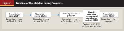
QE1 was announced on November 25, 2008, was expanded in March 2009, and was completed on March 31, 2010 (Da Costa 2011). The focus of QE1 was the purchase of mortgage-backed securities and securities of government-sponsored enterprises (GSEs), such as Fannie Mae, Freddie Mac, and Federal Home Loan Banks securities (Fawley and Neely 2013). Initially, the Fed would buy $600 billion, but it announced in March 2009 that it would purchase another $750 billion in mortgage-backed securities and $175 billion of GSE debt.
QE2 was announced on August 27, 2010. The program started on November 3, 2010 and ended June 30, 2011. Under QE2, the Fed purchased $600 billion of U.S. Treasuries. QE2 was implemented because the Fed feared that the economy was recovering too slowly and that there was a genuine possibility of disinflation. The intention of QE2 was to help lower long-term interest rates and prevent deflation (Fawley and Neely 2013).
During the summer of 2011 and after QE2 had ended, there was a hiatus in Fed programs. Also in the summer of 2011, the U.S economy faced a potential government shutdown because Congress failed to increase the nation’s debt ceiling. Economic data released over the summer of 2011 suggested anemic growth in the United States, including stubbornly high unemployment. In early August 2011, the European sovereign debt crisis resurfaced. Lastly, Standard & Poor’s lowered the credit rating on U.S. government debt partly because of the debt ceiling debate but also because Washington was not able to agree to meaningful spending cuts and revenue increases (Bowley 2011).
Despite the downgrade in the credit quality of U.S. government debt, yields fell rather than rose; however, the United States still remained very attractive to global investors compared to purchasing the debt of other nations (Detrixhe 2011).
Following the economic turmoil in the summer of 2011, the maturity extension program was announced on September 21, 2011. An objective of this program was to not add to the size of the Fed’s balance sheet as the first two rounds of quantitative easing had done. Rather, the Fed would buy longer-term debt (debt with maturities of six to 30 years), and sell shorter-term debt (debt with maturities of three years or less). The Fed would further reinvest principal payments from mortgage-backed securities and agencies into mortgage-backed securities rather than into U.S. Treasuries. The intention of this program was to push longer-term rates down and shorter-term rates up. The maturity extension program was extended on June 20, 2012 and included monthly purchases and sales of $45 billion of securities (Fawley and Neely 2013).
On September 13, 2012, the Fed announced QE3. The program initially began with monthly purchases of mortgage-backed securities in the amount of $40 billion. Simultaneously, the maturity extension program continued. However, on December 12, 2012, the Fed announced that the $45 billion of securities purchases would no longer be offset with sales of short-term securities, effectively ending the maturity extension program. QE3 would include the purchases of $40 billion of mortgage-backed securities and $45 billion of longer-duration U.S. Treasuries, with no offsetting sales of shorter-term U.S. Treasuries (Fawley and Neely 2013). QE3 had no pre-determined ending date.
Methodology
To measure the impact of quantitative easing on the S&P 500 Index, a comparison of the actual market value of the S&P 500 Index—encompassing the time periods during and between quantitative easing programs—was made to estimated market values assuming no quantitative easing programs had occurred.
The study used a variation of the Gordon Growth Model (Damodaran 2012) to derive quarter-end implied required rates of return on the S&P 500 Index for each quarter that spans from Q4 2008 through Q3 2013. Earnings, or the “next period” earnings (earnings for the next 12 months), were a necessary input to the calculations. To determine the “next period” earnings, a growth rate for earnings and dividends was estimated by using the rolling 20-year quarter-over-quarter annualized nominal GDP growth rate.
Quarter-end implied market risk premiums were calculated by subtracting the actual quarter-end 10-year U.S. Treasury bond yield from the implied required rates of return (r). Regression analysis was used to predict the quarter-end yields on the 10-year U.S. Treasury bond had the quantitative easing programs not been implemented. To estimate values of the S&P 500 Index with no quantitative easing programs, the calculated implied market risk premium was added to the predicted 10-year U.S. Treasury bond yield had no quantitative easing programs been in place. That calculation resulted in another implied rate of return (r1) for each quarter-end spanning from Q4 2008 through Q3 2013. The “next period” earnings were divided by the resulting implied rates of return (r1) to estimate an S&P 500 Index value assuming quantitative easing was not in effect.
The focus of the study was to measure the risk-free rate’s effect on equity prices resulting from quantitative easing. There was no attempt made to determine the impact on corporate earnings from quantitative easing. The corporate earnings used for the valuation of the market assuming no quantitative easing programs were actual reported operating earnings. For the purposes of this study, it was assumed that there was a net neutral effect on earnings.
Estimating the Risk-Free Rate Assuming No Quantitative Easing
The key variable that differentiates stock prices with quantitative easing versus stock prices without quantitative easing is the risk-free rate of return on the 10-year U.S. Treasury bond.
It is generally acknowledged that there is a strong relationship between the growth in the economy and interest rates. Based on this premise, regression analyses were used to validate the association between GDP and the 10-year U.S. Treasury bond yield had the quantitative easing programs not been in place. The analysis showed that the rolling 10-year quarter-over-quarter annualized nominal GDP growth rate was associated with GDP over the prior 30 years. As such, the prior 30 years of 10-year U.S. Treasury bond yields was used as the dependent variable. The correlation was 91 percent, the R² was 83 percent, and the t statistic of the correlation coefficient was statistically different from zero.
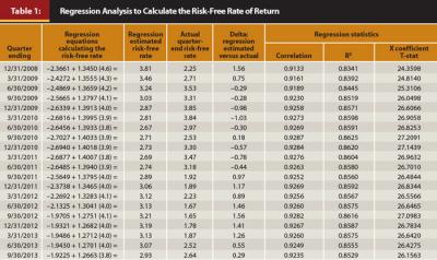
A regression analysis was then run to estimate quarter-end 10-year U.S. Treasury bond yields beginning with the yield for Q4 2008. The regression analysis was then re-calculated every quarter going forward from Q1 2009 through Q3 2013. Each quarterly yield calculated was used in the later calculation of quarterly market values assuming no QE programs were in place.
To estimate the 10-year U.S. Treasury bond yield in effect for Q4 2008, the independent variable in the regression analysis used the prior 30 years of rolling 10-year quarter-over-quarter annualized nominal GDP growth rate data starting with Q4 1978 and ending with Q3 2008. The data point for Q4 1978 reflected the average of the prior 10 years of quarterly, quarter-over-quarter annualized nominal GDP data, starting with Q1 1969. The dependent variable used the observed prior quarter-end yields for the 10-year U.S. Treasury bond. Each yield, starting with Q4 1978 going forward to Q3 2008, was used in the regression analysis for Q4 2008.
The regression generated and used to estimate Q4 2008 10-year U.S. Treasury bond yield was as follows: 3.81 = –2.3661 + 1.3450 (4.6).
The 3.81 represents an estimated 3.81 percent 10-year U.S. Treasury bond yield for Q4 2008. The intercept term is –2.3661, and the X variable coefficient is 1.3450. The 4.6 is the independent variable, which represents the actual rolling 10-year quarter-over-quarter annualized nominal GDP as of Q4 2008.
To estimate Q1 2009, the 30 years of rolling 10-year quarter-over-quarter annualized nominal GDP growth rate data were used, starting with Q1 1979 through Q4 2008. In the regression analysis, to estimate the 10-year U.S. Treasury bond yield for Q1 2009, the prior 30 years of 10-year U.S. Treasury bond yields included the estimated 3.81 percent for Q4 2008, not the actual 10-year U.S. Treasury bond yield of 2.25 percent. Going forward, as each quarterly yield was estimated, the projected yield was then included in the 30 years of sample data used as the dependent variable.
In each new regression equation, the independent variable was inserted into the equation to calculate an estimated yield on the 10-year U.S. Treasury bond yield for each respective quarter-end going forward.1 Results are shown in Table 1.
A conclusion from the study of relationships of nominal GDP growth rates and 10-year U.S. Treasury bond yields is that the 10-year U.S. Treasury bond yield reflects the long-run growth rate in the economy. That is, the high readings of the correlation and R² of the 10-year U.S. Treasury bond yield to the nominal GDP growth rate suggest that slower growth in the economy over any prior 10-year period is reflected in lower yields, while a faster growth rate over any prior 10-year period is followed by a higher yield. A pattern of slower long-term (over 10 years) growth in nominal GDP should be followed by lower relative 10-year U.S. Treasury bond yields. Faster long-term average growth in nominal GDP should be followed by higher relative yields.
Estimating the Required Rate of Return and Market Risk Premium
Damodaran (2012) suggested three methods for calculating the required return on equities and the market risk premium: (1) the survey method, (2) the historical method, and (3) the implied required return and equity risk premium approach.
The survey method is what other investors, CFOs, and academics estimate. The historical method takes the average of the return on the market less the return of the risk-free rate over a specified time period. The disadvantage associated with this method is that it is backward-looking and assumes that the past is the best indication of the future. According to Damodaran, most investors use this method.
The third method calculates an implied required rate of return and equity premium. The implied required return and equity premium approach is a variation of the stable growth dividend discount model or Gordon Growth Model. This is the approach chosen for this study, primarily because it is considered to be more forward-looking and because it is more objective than the survey method.
Damodoran’s (2012) variation to the Gordon Growth Model focuses on earnings rather than dividends to calculate the value of an equity. The model variation is used to solve for the implied required return on equity as follows:
Gordon Growth Model:
Value of an equity =
Expected dividends next period
-----------------------------------------------
Required rate of return – growth
rate of earnings and dividends
Gordon Growth Model Variation:
Value of an equity =
Expected earnings next period
------------------------------------------------
Required rate of return
where,
Required rate of return=
Expected earnings next period
----------------------------------------------- =
Value of equity
Earnings (E)
-----------------------
Price (P)
The earnings yield ( (E)/(P) ) is characterized as the implied required rate of return (Damodaran 2012). In the study, the implied required rate of return (r) was the earnings yield on the S&P 500 Index. The equity risk premium was derived by taking the resulting required return on equities and subtracting the risk-free rate of return. The risk-free rate was defined as the 10-year U.S. Treasury bond yield.2 The implied market risk premiums, as shown in Table 2, were found by rearranging the capital asset pricing model (CAPM) to solve for the market risk premium as follows:
CAPM = r = Risk free rate + (β x market risk premium
where,
β = beta = 1.0
Market risk premium = r – risk-free rate
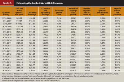
The market risk premium was then recalculated for each quarter for the duration of the study. After the implied market risk premium was calculated for each quarter, it was added to the regression estimated yield for the 10-year U.S. Treasury bond yield to obtain a new required rate of return (r1) for each quarter from Q4 2008 through Q3 2013 using the following formulas:
New required rate of return (r1) = Market risk premium + Regression estimated risk-free rate
New required rate of return (r1) = Earnings yield on S&P assuming no quantitative easing
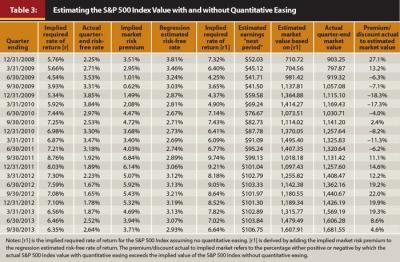
The resulting required rate of return (r1) calculated for each quarter was used as the earnings yield for the S&P 500 Index for a market assuming no quantitative easing. The estimated market value assuming no quantitative easing was then derived by dividing the estimated earnings “Next Period” by the implied required rate of return (r1) (Table 3).
Estimating the Growth Rate in Earnings and Dividends
An estimated stable growth rate for earnings and dividends was used to calculate the “next period earnings” or earnings for the next 12 months. The variation of the Gordon Growth Model, as described earlier, uses the earnings expected in the next 12 months as the formula numerator. McGowen (2012) suggested using a 20-year average of the annual change in nominal GDP growth as an estimate of the long-run growth rate of a mature company. A similar method for calculating the long-term growth rate was used within the study. Because this study values an equity index dominated by many mature companies, a growth rate representative of the economy was used.
The growth rate used in the study was the estimated rolling 20-year quarter-over-quarter annualized nominal GDP growth rate. Going forward, a unique growth rate was calculated for each quarter from December 2008 through September 2013 using the respective rolling 20-year quarter-over-quarter annualized nominal GDP growth rate for each quarter. This calculation of the growth rate of earnings and dividends is separate from, and unrelated to, the calculation earlier of nominal GDP growth rate used in the regression analysis.
Observations and Interpretation of the Study’s Results
Analysis of the data shows that QE1 had little, if any, impact on long-term interest rates. Upon the announcement and commencement of QE1, the 10-year U.S. Treasury bond yield fell initially below 3 percent but rose above 3 percent by the end of Q2 2009. The yield remained above the regression estimated 10-year U.S. Treasury bond yield for the duration of QE1.
The initial drop in the 10-year U.S. Treasury bond yield below the regression estimated yield may have been more a response to the financial crisis that began in the fall of 2008 than any response to the Fed’s actions as investors moved toward the safety of government bonds. With the focus on purchasing mortgage-backed securities and GSEs, the most noticeable impact of the Fed’s actions was seen in mortgage interest rates, as the Fed had intended. At the beginning of QE1 in November 2008, the 30-year fixed rate mortgage rate was 6.33 percent. By the end of QE1 on March 31, 2010, the 30-year fixed-rate mortgage had fallen to 5.23 percent (Da Costa 2011).
A plausible explanation for the actual 10-year U.S. Treasury bond’s yield being higher than the regression estimated bond yield after Q1 2009 may be the result of an increased supply of government debt as the U.S. budget deficit increased dramatically. For fiscal year ending September 30, 2007, the federal budget deficit was $160.7 billion. At the end of fiscal year 2008, the federal budget deficit was $458.6 billion. By end of fiscal year 2009, the federal budget deficit was reported at $1.413 trillion, an increase of 208 percent year-over-year.
Engen and Hubbard (2004) found, through their research, that a 1 percent increase in the federal debt, as a percentage of GDP, was predictive of an increase in long-term interest rates of three basis points. The higher annual budget deficit for fiscal year 2009, compared to fiscal year 2008, contributed to the increase in federal debt as a percentage of GDP. At the end of fiscal year 2008, federal debt as a percentage of GDP was 67.5 percent. This rose to 82.8 percent at the end of fiscal year 2009. At the end of fiscal year 2007, federal debt as a percentage of GDP was 61.8 percent, according to 2013 data from the Federal Reserve Bank of St. Louis.
The stock market began its turnaround on March 9, 2009 when the S&P 500 Index reached its lowest level of the financial crisis. Despite rising interest rates, stocks continued to rise throughout 2009.
The methodology used to compare the market value with quantitative easing to the estimated value of the market assuming no quantitative easing suggests that the higher budget deficits, along with higher corresponding yields on the risk-free rate, adversely affected equity prices as yields were higher than projected through the regression analysis. Assuming the regression estimated yield was the “normal” yield, had the regression estimated yields prevailed during QE1, the S&P 500 Index would likely have been higher as seen by the discounted actual market values to the estimated market values (see Table 3). In other words, had no quantitative easing been in effect, and the federal budget deficits not “abnormally” resulted in nearly a $1 trillion additional supply of government debt from the prior year, the S&P 500 Index might have appreciated even more than it did.
Despite the consistent discounts of the actual market value to the market value without quantitative easing, the S&P 500 Index continued to rise. This increase was supported by growing corporate earnings.
The 10-year U.S. Treasury bond yield began to fall prior to the beginning of QE2. Fawley and Neely (2013) pointed out that it is important to note the movement of interest rates at a program’s announcement, rather than when a program is in effect, to see the full extent of the policy decision’s impact. They pointed out that the 10-year U.S. Treasury bond yield rose after the commencement of QE2 following the yield falling shortly after the original announcement that the Fed would initiate QE2.
The QE2 program was announced on August 27, 2010 but did not commence until November 3, 2010. From August 27, 2010 through October 8, 2010 the 10-year U.S. Treasury bond yield fell by 25 basis points. By November 3, 2010, the yield had increased 26 basis points from the October 8, 2010 low yield. The yield on the 10-year U.S. Treasury bond was 2.67 percent on November 3, 2010 and had risen to a high of 3.75 percent on February 8, 2011 and ended QE2 on June 30, 2011 at 3.18 percent.
Although QE2 focused on purchasing U.S. Treasury bonds rather than mortgages, yields on the 10-year U.S. Treasury bond were higher than those estimated through the regression analysis. Again, the U.S. budget deficit continued to be at a higher dollar level than it had ever been historically. The higher yields suggest a greater supply of U.S. Treasuries issued to the market. This may have contributed to upward pressure on yields.
The budget deficit was $1.294 trillion for fiscal year 2010. The S&P 500 Index continued to rise, supported by growing corporate earnings. The higher actual yields, versus the regression estimated yields, during QE2 suggest that the S&P 500 Index was held back by the higher risk-free rate and could have advanced further had the actual risk-free rate been as low as the regression estimated yield. The comparison of the actual market values versus the non-quantitative easing market values shows that the actual market value with quantitative easing sold at a discount to the estimated market value assuming no quantitative easing from Q4 2010 through Q2 2011 (Table 3).
In the summer of 2011, yields on the 10-year U.S. Treasury bond remained above the regression estimated yield. The actual yield peaked on July 1, 2011 at 3.22 percent, while equity prices peaked on July 22, 2011. As a result of the aforementioned events in Europe and Washington in the summer of 2011, the yield gradually fell throughout the summer without any Fed program in place. Equity prices also dropped as a result of the summer of 2011 turmoil. The yield remained low and equity prices began to recover from the selloff over the summer of 2011 without the assistance of a quantitative easing program from the Fed.
On September 21, 2011, following the Federal Open Market Committee (FOMC) meeting, the Fed announced the commencement of the maturity extension program. By September 21, 2011, the 10-year yield had fallen to 1.88 percent, which was below the regression estimated yield. This occurred not because of quantitative easing (the maturity extension program had just started) but rather because of the turmoil in the summer of 2011.
After the commencement of the maturity extension program, and subsequently QE3, the yield sustained a level below the regression estimated yield. The design of the maturity extension program, which entailed selling short-term government securities and buying intermediate-term bonds, had the effect of lowering the yield on the 10-year U.S. Treasury bond and would likely have lowered the yield even if the summer of 2011 had been uneventful. Comparing the S&P 500 Index valuation with quantitative easing to the S&P 500 Index valuation estimated without quantitative easing, this study suggests that at the end of September 2011, the market with quantitative easing had a premium of 11.1 percent over the market assuming no quantitative easing (the S&P 500 Index fell 16.4 percent from July 7 through September 30, 2011).
At the same time the maturity extension program began, the U.S. budget deficit for fiscal year ending September 30, 2011 was nearly $1.3 trillion, which was slightly higher than the prior year’s budget deficit. Despite the high budget deficit and corresponding supply of U.S. Treasury debt, yields fell, suggesting the scope of the maturity extension program (selling shorter-term debt and buying longer-term debt with the proceeds) had a meaningful impact on yields. The impact was large enough to offset the continuing high supply of government debt hitting the market. For the quarter ending September 30, 2011, the yield on the 10-year U.S. Treasury bond had fallen to 1.92 percent versus the regression estimated yield of 2.89 percent.
As market volatility subsided after the summer of 2011, the impact of the maturity extension program on the S&P 500 Index became more apparent. Using the methodology to compare the S&P 500 Index valuation with the maturity extension program to the S&P 500 Index valuation assuming no quantitative easing market, this study suggests that the market with the maturity extension program had a premium of 14.6 percent over the market value assuming no quantitative easing as of the end of 2011. Further, comparing the premium on the S&P 500 Index with the maturity extension program over the market, assuming no quantitative easing, increased to 19.2 percent by the end of June 2012 (Figure 2).
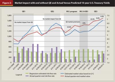
The premium climbed to as high as 22 percent for the quarter ending September 2012 at the same time that QE3 began. The maturity extension program and the QE3 program overlapped through the end of 2012, and the premium remained high at 19.9 percent (Table 3). As the maturity extension program was winding down and ending at the end of 2012, the premium also began to fall.
From the commencement of QE3, the yield on the 10-year U.S. Treasury bond remained well below the regression estimated yield until the Fed meeting on May 22, 2013 when the Fed hinted at “tapering” easing policy. Tapering refers to the Fed’s intended reduction in purchases of Treasuries or mortgage-backed securities from the then current level of $85 billion total per month. The market began to price in tapering based on the Fed’s statements as yields on the 10-year U.S. Treasury bond rose sharply from May 22, 2013 through September 18, 2013.
The Fed members agreed not to taper at the September FOMC meeting. The yield on the 10-year U.S. Treasury bond began to fall as the effects of the anticipated Fed actions did not materialize. However, the market did not fully unwind its pricing of the effects of tapering.
Finally, as a result of the tapering talks by the Fed and subsequent rise in the yield on the 10-year U.S. Treasury bond, the premium between the actual value of the S&P 500 Index to the estimated value of the S&P 500 Index with no quantitative easing began to fall. At the end of June 2013, the premium had fallen from 19.3 percent at the end of March 2013 to a premium of 8.6 percent. As the yield continued to rise, the premium fell to 4.6 percent at the end of September 2013. The implication of a rising yield is that as the yield increases toward the regression estimated yield, equity prices converge toward their estimated valuations assuming quantitative easing not been in place. Thus, the measurable impact of quantitative easing does not seem to be sustainable beyond the duration of the quantitative easing programs.
Implications for Planners
The Fed began to taper quantitative easing prior to the end of former Chairman Ben Bernanke’s term and before he handed off the Chair to Janet Yellen. Although Yellen is considered by many to be “dovish,” financial planners should assume that she will continue the tapering of quantitative easing as initiated by her predecessor until the current program is ended.
As the tapering of quantitative easing occurs, planners may want to assume that there will only be modest upward pressure on interest rates as a result of the Fed’s tapering as, it is argued, tapering effectively began after the May 2013 FOMC meeting. Interest rates will be less influenced by quantitative easing and more affected by the fundamentals of the economy.
Likewise, planners may want to assume that going forward, Fed tapering will have little adverse effect on equity prices, because much of the premium of the S&P 500 Index with quantitative easing, compared to the estimated S&P 500 Index without quantitative easing, had disappeared as the S&P 500 Index sold off following both the May 2013 and June 2013 FOMC meetings. Equity market valuations will likely be more influenced by fundamentals going forward than by the Fed’s pace of tapering and eventual completion of the quantitative easing programs.
Conclusion
The methodology employed in this study compared the S&P 500 market value with quantitative easing to the market value had there been no quantitative easing. This analysis was made in order to measure the impact quantitative easing had on the S&P 500 Index. Both QE1 and QE2 had no measurable impact on equity prices. QE1 focused on mortgages and GSEs, not Treasuries. Both QE1 and QE2 met the offsetting impact of large federal budget deficits, which may otherwise have resulted in pressure on U.S. Treasury yields.
The study demonstrated that the subsequent maturity extension program and QE3 had a measurable impact on equity prices. The study showed that the S&P 500 Index experienced a maximum premium of 22 percent at the end of September 2012, compared to the S&P 500 Index with no quantitative easing. The maximum impact on equity prices was observed when both the maturity extension and QE3 programs were in effect simultaneously.
The beginning of the end of quantitative easing actually commenced with the Fed’s statement following its FOMC meeting on May 22, 2013, although the Fed continued to buy $85 billion of securities each month. The Fed’s taper talk at the May and June FOMC meetings effectively began the upward move of interest rates toward the regression estimated yields. Finally, any effects on the equity market valuations are not likely sustainable beyond the ending of the quantitative easing programs. The market valuations assumed both with and without quantitative easing began to converge as actual yields moved toward estimated yields.
Endnotes
- Other relationships of GDP data were also tested to determine which would provide the “best” relationship to the 10-year U.S. Treasury bond yield. Twenty, 25, and 40 years of data were also used. In addition to 10-year rolling data, three-, five- and seven-year rolling data were used over the previous 40 years. These combinations had very high correlations and R² readings, but not as high as the 10-year rolling data over the prior 30 years. Quarterly (non-rolling), quarter-over-quarter annualized nominal GDP data were also incorporated into the analysis, but these had minimal correlation and R² compared to the 10-year U.S. Treasury bond yield. Although the testing of relationships was not exhaustive, there was sufficient confidence in the relationship chosen for the study.
- The 10-year bond yield was used because it is a long-term rate and equities are a long-term investment. Had the analysis valued a short-term investment, such as a stock option as used in the Black Sholes model, a six- or three-month bill rate would be desirable.
References
Bowley, Graham. 2011. “Stocks Plunge on Fears of Global Turmoil.” The New York Times August 4.
Da Costa, Polyana. 2011. “End of QE1: Financial Crisis Timeline.” Bankrate.com.
Damodaran, Aswath. 2012. Equity Risk Premiums (ERP): Determinants, Estimation and Implications (2012 Ed., pp. 16–21, 61–64).
Detrixhe, John. 2011. “U.S. Loses AAA Credit Rating as S&P Slams Debt Levels, Political Process.” Bloomberg.com.
Engen, Eric, and R. Glenn Hubbard. 2004. “Federal Government Debts and Interest Rates.” National Bureau of Economic Research.
Fawley, Brett W., and Christopher J. Neely. 2013. “Four Stories of Quantitative Easing.” Federal Reserve Bank of St. Louis Review 95 (1): 51–88.
McGowan Jr, Carl B. 2012. “Determining the Long-Term Growth Rate for Common Stock Valuation.” The 2012 Orlando International Academic Conference: 617–620.
Citation
Olsen, James L. 2014. “The Impact of Quantitative Easing on Equity Prices.” Journal of Financial Planning 27 (5): 52–60.