HECM Reverse Mortgages: Now or Last Resort?

Journal of Financial Planning; May 2014

 

Shaun Pfeiffer, Ph.D., is an associate professor of finance and personal financial planning at the Edinboro University of Pennsylvania.

C. Angus Schaal, CFP^®, is founder and senior managing director of Tandem Wealth Advisors in Phoenix, Arizona.

John Salter, Ph.D., CFP^®, AIFA^®, is an associate professor of personal financial planning at Texas Tech University and a wealth manager at Evensky & Katz Wealth Management in Coral Gables, Florida, and Lubbock, Texas.

Executive Summary

• This study outlines recent changes in the reverse mortgage market and investigates plan survival rates for distribution strategies that establish a Home Equity Conversion Mortgage (HECM) reverse mortgage line of credit at the beginning of retirement and as a last resort. 
• Calculations were based on Monte Carlo simulations using a 4 percent to 6 percent real withdrawal rate, in 1 percent increments, for a client who has a $500,000 nest egg and $250,000 in home equity at the beginning of retirement. The nest egg was split into a 60 percent stock and 40 percent bond investment portfolio alongside a six-month cash reserve. 
• Results are shown for scenarios where the HECM line of credit is established during: (1) low interest rates at age 62, (2) low interest rates when the investment portfolio is exhausted, (3) moderate interest rates when the investment portfolio is exhausted, and (4) high interest rates when the investment portfolio is exhausted.
• Early establishment of an HECM line of credit in the current low interest rate environment is shown to consistently provide higher 30-year survival rates than those shown for the last resort strategies. The early establishment survival advantage for real withdrawal rates at or above 5 percent is estimated to begin between 15 and 20 years after loan origination and is shown to be as high as 31 percentage points, or 85 percent, greater than the last resort survival rates.

Many retirees and advisers resisted reverse mortgages in the past because of high costs (Chiuri and Jappelli 2010). However, research such as Boston College’s National Retirement Risk Index 2010, has noted that many future retirees will not be in a position to avoid using home equity in retirement. Other research has shown that seniors will increasingly turn to reverse mortgages, because more affordable reverse mortgage options are now available than in the past (Timmons and Naujokaite 2011). If more seniors consider reverse mortgages, a number of these retirees are likely to seek advice on whether to establish the reverse mortgage now, or later as a last resort. 

This study outlines recent changes in the reverse mortgage market and attempts to shed light on two simple questions: (1) which client-specific and capital market factors should a practitioner emphasize; and (2) based on these critical factors, how does early or delayed establishment influence whether a reverse mortgage can improve the probability of clients’ maintaining their retirement spending goals?

The intent of this study is not to determine if someone should establish a reverse mortgage. Rather, if maintaining a client’s real income needs is to require the use of home equity, then what factors should be considered, and how do these factors impact whether a reverse mortgage should be established now or as a last resort? 

The motivation for this investigation stems from concerns associated with delayed establishment of reverse mortgages noted by Kitces (2011). The present work is closely related to Sacks and Sacks (2012), which explored the use of the Home Equity Conversion Mortgage (HECM) Standard (which is no longer available) and found that earlier establishment of the reverse mortgage consistently led to a higher likelihood of goal attainment than seen under last resort establishment scenarios.

This study expands on the existing literature by comparing the efficacy of early versus last resort establishment of the new HECM line of credit. The early establishment strategy in this study is based on a passive approach where the HECM line of credit is only used if and when the investment portfolio is exhausted, whereas the Sacks and Sacks study examined two active approaches where the line of credit was used from the onset of retirement. In addition, this study sheds light on the importance of expected home ownership duration, interest rates, and home appreciation when a reverse mortgage is being considered. 

The empirical results from this analysis suggest early establishment of an HECM line of credit in the current interest rate and lending environment consistently provides greater survival rates than those strategies where the line of credit is established after the investment portfolio is exhausted. We estimate that the realization of the early establishment survival advantage over last resort establishment begins to appear between 15 and 20 years after the loan origination date for real annual withdrawal rates at or above 5 percent.

Further, early establishment survival rates are estimated to be as high as 85 percent, or 31 percentage points, greater than the last resort survival rates at the 30th year in retirement. In other words, expected home ownership duration is an important element in determining whether early establishment of a reverse mortgage is an appropriate strategy.

In addition, the early establishment survival advantage in the current interest rate and lending environment is estimated to be greatest for those who expect (1) long duration of home occupancy, (2) higher real withdrawal needs relative to home value, (3) higher future interest rates, and (4) lower future home appreciation.

HECM Background and Review 

A new HECM product replaced the HECM Standard and Saver on September 30, 2013 (U.S. Department of Housing and Urban Development 2013). The HECM program was introduced in the Housing and Community Development Act of 1987 (Consumer Financial Protection Bureau 2012, p. 153) and is estimated to account for more than 90 percent of the reverse mortgage market. The new legislation gave authority to the Department of Housing and Urban Development (HUD) to administer the program and for the Federal Housing Administration (FHA) to insure HECM reverse mortgages.

The new HECM reverse mortgage represents a blend of the HECM Saver and Standard products; however, the upfront mortgage insurance premium (MIP) has been changed, and the amount of home equity that can be used within the first year after loan origination has been capped at 60 percent. A comparison of the new HECM and discontinued HECM Saver and Standard programs is presented in Table 1.

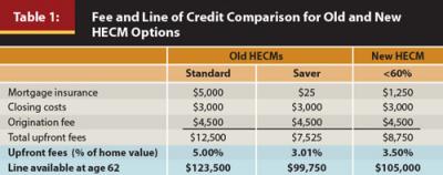
Table 1 illustrates the difference in total upfront fees and the maximum line of credit available to a 62-year-old borrower with a $250,000 home value and no mortgage debt at loan origination (with upfront fees paid from the portfolio). This example also assumes a 3 percent lender’s margin¹ and a 3 percent 10-year Libor swap rate.² Total upfront fees consist of a MIP, closing costs, and origination fees. Servicing fees may be assessed by the lender if not already accounted for in the upfront and ongoing interest rates charged to the borrower. Escrow reserves may be required and are contingent upon lender requirements based on financial information of the borrower (Munnell and Sass 2014). 

For this example, the only difference in upfront fees is the MIP, which is set by the FHA and was 2.0 and 0.01 percent of the home value for the HECM Standard and Saver, respectively. The new HECM has a 0.5 percent MIP, so long as less than 60 percent of available proceeds are used within the first year. The total upfront fees for a new HECM (see Table 1) are roughly 16 percent, or 0.49 percentage points higher than the discontinued Saver, and roughly 30 percent, or 1.5 percentage points lower than the discontinued Standard.

The bottom row of Table 1 shows the available line of credit for the new HECM. This is roughly 5 percent higher than the line of credit for the Saver, and 15 percent lower than the line of credit for the Standard. In short, the new HECM is not meaningfully different from the HECM Saver product if the borrower does not use 60 percent or more of the line of credit in the first year after loan origination. If the borrower uses more than 60 percent of the line of credit in the first year, the upfront MIP cost is 2.5 percent, rather than 0.5 percent.

It is important to note that the figures provided in Table 1 are based on the maximum allowable origination fee set by HUD. Further, closing costs are set at the top of the expected range provided in a report by AARP (2011). In addition to upfront fees, ongoing interest consists of a variable interest rate that changes monthly, the lender’s margin set at date of origination, and an annual 1.25 percent MIP charged by FHA. The variable interest rate is indexed to the one-month Libor rate,³ and, as of December 2013, is 0.2 percent. This variable rate is adjusted monthly.

In today’s environment, a borrower would initially face a total annual effective interest rate of 4.45 percent, if the lender’s margin is 3 percent. Roughly one-twelfth of this rate accrues to any outstanding loan balance and unused portion of the line of credit on a monthly basis. The available line of credit, holding age of the borrower constant, increases as interest rates decrease.

A commonly overlooked advantage of establishing a line of credit early is the growth of the unused line of credit. The annual growth rate that applies to the unused line of credit is a constant 4.25 percent plus the variable one-month Libor rate, which has ranged from 0.2 percent to 7.0 percent since 2000. Upfront and ongoing interest is incurred by the borrower in exchange for access to home equity.

The principal limit factor (PLF) represents the percent of home equity that is available in the form of a line of credit and is published by HUD. The age of the youngest borrower, and the expected interest rate at loan origination, determine the PLF. The expected interest rate is the summation of the 10-year Libor swap rate and the lender’s margin. The PLF increases with age and decreases when expected interest rates rise. As of December 2013, the 10-year Libor swap rate was 3 percent. Therefore, a 62-year-old borrower who is assessed a 3 percent lender’s margin would receive a line of credit equal to 42 percent ($105,000) for a mortgage-free $250,000 home under the new HECM. These figures also assume that all upfront fees are paid out of pocket. 

Considerations for the HECM Today

As more seniors are forced to consider reverse mortgages, some are likely to seek advice on whether they should establish one now, or later as a last resort. Historically, the conventional wisdom in financial planning circles viewed the use of reverse mortgages as a last resort (Sacks and Sacks 2012). The evolution of the reverse mortgage market led some notable financial planners and researchers to question the validity of the conventional wisdom.

For example, Kitces (2011) noted that the appeal of using a reverse mortgage from the onset of retirement had increased due to the introduction of a more affordable reverse mortgage option known as the HECM Saver. A similar perspective on the HECM Saver was offered by Harold Evensky (Schulaka 2013). However, discussion and existing research on the new HECM is limited. Two recent studies outlined the potential benefits of the new HECM (Pfeiffer, Salter, and Evensky 2013; Wagner 2013), but left the comparison of early versus last resort establishment for future study. 

A number of factors should be evaluated prior to determining whether a reverse mortgage is appropriate and, if at all, when it should be established.

The youngest borrower must be at least 62 in order for the household to qualify for a reverse mortgage. The amount of home equity that can be accessed increases with the age of the youngest borrower. Even with the increase, research has indicated that establishing a reverse mortgage at younger ages is generally preferable to waiting (Sacks and Sacks 2012).

Sun, Treist, and Webb (2007) noted increasing interest rates, the potential for a decrease in home value, and uncertainty associated with the lending environment and product design as significant risks associated with delayed establishment of a reverse mortgage. In addition, the ability to amortize costs over a longer period, and mitigate the potential detrimental impact of sequence of return risk, also support early establishment of a reverse mortgage (Kitces 2011; Salter, Pfeiffer, and Evensky 2012).

The expected duration of home occupancy after loan origination is another factor that should be considered when determining the timing and appropriateness of establishing a reverse mortgage. Borrowers who expect to stay in their home for an extended period of time are likely to benefit more from earlier establishment of a reverse mortgage, so long as the interest rate and lending environment are reasonable. It has been noted that HECMs have “historically offered borrowers favorable pricing” (Davidoff 2013, p. 1), and that the current low interest rate environment allows reverse mortgage borrowers to access higher levels of home equity when compared to higher interest rate environments (Kitces 2011). 

Existing studies have accounted for various interest rates, home appreciation, and other relevant factors, and have collectively reported significant survival advantages associated with the use of reverse mortgages. For example, studies centered on the HECM Standard and Saver products found that early establishment and sound use of reverse mortgages can reduce shortfall risk at the 30-year mark in retirement by as much as 50 percent when compared to distribution strategies that fail to use a reverse mortgage (Sacks and Sacks 2012; Salter et al. 2012).

More recent studies focused on the new HECM have shown that the sustainable withdrawal rate could be increased to approximately 6 percent for a 30-year retirement (Pfeiffer et al. 2013; Wagner 2013). However, the existing literature fails to provide an extensive analysis on early establishment of the new HECM compared to establishing an HECM as last resort. In addition, the existing literature has failed to examine the impact of expected home ownership duration, and various interest rate and home appreciation scenarios, despite the noted importance of these factors (Kitces 2011; Sun et al. 2007). 

Methodology 

This study compares the efficacy of two simple strategies: (1) establish an HECM line of credit at age 62, under the current lending and interest rate environment, and do not use the HECM line of credit until the investment portfolio is exhausted; or (2) wait until the investment portfolio is exhausted, if ever, and establish an HECM line of credit on that date and subsequently begin to use the proceeds to support income needs until the line of credit is exhausted.

The first strategy (now–low) is viewed from the current low interest rate environment.⁴ However, the second strategy is viewed from three different possible future interest rate environments. Monte Carlo analysis using 10,000 simulations was used to estimate plan survival rates and median wealth for each of four unique distribution scenarios, in which the HECM line of credit is established during: 

• Low interest rates at age 62 (now–low)
• Low interest rates when the investment portfolio is exhausted (late–low)
• Moderate interest rates when the investment portfolio is exhausted (late–mid)
• High interest rates when the investment portfolio is exhausted (late–high)

The now-low scenario is based on a client who establishes an HECM line of credit at age 62, when the 10-year Libor swap rate and lender’s margin are 3 percent, and the initial line of credit is $105,000 or 42 percent of a home’s $250,000 value.

Each of the last resort scenarios, prefixed by the term “late,” establishes the line of credit later in retirement after the investment portfolio has been exhausted. The lender’s margin is set at 3 percent, whereas the 10-year Libor rate at loan origination date is 3 percent, 5 percent, or 7 percent for the late–low, late–mid, and late–high scenarios, respectively.

The initial line of credit for each of these last resort scenarios is different because of the variability in age at which the investment portfolio is exhausted for a given simulation. For example, a simulation where the investment portfolio is exhausted at age 80, the line of credit would be 53.1 percent, 42.5 percent, and 34.2 percent of the home value for the late–low, late–mid, and late–high scenarios, respectively.

Scenario results are shown for a 4 percent to 6 percent real withdrawal rate in 1 percent increments, and for zero and 2 percent real annual home appreciation rates. Each scenario is also based on a client who has a $500,000 nest egg and $250,000 in home equity at the beginning of retirement. The nest egg is split into a 60 percent stock and 40 percent bond investment portfolio alongside a cash reserve equal to six months of real retirement income needs. Each of the Monte Carlo simulations represents a hypothetical economic environment during retirement with different investment portfolio return patterns and interest rates. Each simulation incorporates up to 420 months’ (35 years’) worth of information on investment returns, interest rates, volatility, and transaction costs. 

Income needs are met by using the cash reserve account. The cash reserve account is refilled by the investment portfolio until it is exhausted. Thereafter, the cash reserves are refilled by the HECM line of credit if the balance dips below two months’ worth of forward- looking real withdrawal needs. In addition, the cash reserve is refilled if there is a need to rebalance and at least one of the asset class’s prior year returns is positive. If prior year returns for both asset classes are negative, withdrawal needs exceed two months’ worth of needs, and there is a need to rebalance, then the portfolio will be rebalanced; however, no cash refill will occur due to the potential of selling a depreciated asset. 

Capital Market Assumptions

This study assumes an average annual nominal pre-tax return of 8.75 percent for stocks, 4.75 percent for bonds, and 3.50 percent for cash. The assumed annualized standard deviation is 21.0 percent, 6.5 percent, and 2.0 percent for stocks, bonds, and cash, respectively. Correlation of stocks to bonds was modeled at 30 percent. These return and volatility assumptions are in line with the latest forward-looking projections provided by MoneyGuidePro software and are similar to low return projections seen in Arnott and Bernstein (2002) and Cornell (2010). Transaction costs are set at $30 per trade, and taxes are not accounted for in the analysis. Rebalancing back to the initial allocation occurs when one of the asset classes deviates by 5 percent or more, in absolute terms, from the policy allocation. 

Ongoing interest rates, home appreciation, and inflation assumptions are modeled as follows. First, note that the 10-year Libor swap rate, as discussed previously, is only applicable to the loan origination date. The one-month Libor rate adjusts monthly and represents the ongoing interest rate that, when added to the constant lender’s margin and annual MIP, accrues to any outstanding loan balance and/or increases the unused portion of the line of credit.

Wagner (2013) reported that the HECM program uses the 10-year Libor rate as the proxy for the next 120 months of one-month Libor rates. Therefore, we used the 10-year Libor rate at the loan origination date as the projected one-month Libor rate for the first 10 years after loan origination. This leads to a projected one-month Libor rate of 3 percent, 5 percent, and 7 percent for the first 10 years after the loan origination date for each of the unique interest rate scenarios.

Next, we used the median one-month Libor rate of 5 percent and 2.5 percent standard deviation (based on data from January 1986 through December 2013) to project subsequent one-month Libor rates in each interest rate scenario. The inflation assumption is constant at 3 percent in nominal terms per year, whereas home appreciation is either a constant zero or 2 percent in real terms per year.

The lender’s margin and annual ongoing MIP are assumed to be constant at 3 percent and 1.25 percent per year, respectively. Upfront costs are assumed to be 3.5 percent of the home value on the loan origination date, and a $35 monthly service fee (adjusted for inflation) is subtracted from the investment portfolio or available line of credit each month. All upfront fees are paid from the investment portfolio in the early establishment strategy, whereas last resort strategies fees are financed since the investment portfolio and cash reserves are exhausted at the date of loan origination.

Finally, unlike assumptions in some existing studies, the simulations in this study do not use the line of credit to fund needs during bear markets when the investment portfolio has not yet been exhausted. This study assumes the line of credit is set in the early establishment strategy and is left unused until the investment portfolio has been exhausted. Note that the unused portion of the line of credit grows at one-twelfth the summation of lender’s margin, annual MIP, and one- month Libor rate each month.

Results

Survival rates and median wealth for the 10th, 20th, and 30th year in retirement are shown for each of the four distribution strategies in Table 2. The results are based on a client who begins retirement at age 62, has a $500,000 nest egg, $250,000 in home equity, and either establishes a reverse mortgage at age 62 (now–low), or establishes the reverse mortgage as a last resort in retirement. Each of the last resort scenarios is prefixed by the term “late” followed by the level of interest rates at loan origination date when the investment portfolio is exhausted. Panel A in Table 2 reports survival and median wealth for a retiree who experiences real annual home appreciation of zero percent, whereas Panel B is associated with real home appreciation of 2 percent per year.

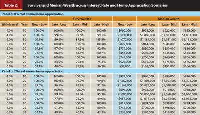
Survival results in Table 2 associated with real withdrawal rates at or above 5 percent suggest that early establishment of the HECM line of credit (now–low) consistently leads to higher survival rates in years 20 and 30 of retirement, when compared to survival rates for each of the three last resort establishment scenarios. The early establishment survival advantage over each of the last resort approaches is shown to increase with the real withdrawal rate, year in retirement, and higher realized interest rate at future loan origination date. However, the early establishment survival advantage is not realized for any of the real withdrawal rates or home appreciation scenarios at the 10th year in retirement. In other words, more than 10 years after loan origination must elapse before survival benefits associated with early establishment begin to appear. This observation holds true for each of the different real withdrawal and home appreciation assumptions.

Finally, a comparison of Panel A to Panel B shows that the early establishment survival advantage over last resort establishment is higher when lower home appreciation is experienced after loan origination date. 

Median wealth for a given year and scenario, across all simulations, is also shown in Table 2. Wealth is calculated by taking the greater of $0 or home value minus any outstanding loan balance plus the investment portfolio and cash reserves. The nonrecourse attribute of HECM reverse mortgages holds HUD’s insurance fund responsible for loan balances in excess of the home value. Median wealth results suggest that early establishment of the HECM line of credit consistently leads to lower median wealth than seen with each of the three last resort establishment scenarios. The estimated reduction in median wealth for early establishment in relation to each of the last resort approaches is also shown to increase with the real withdrawal rate and year in retirement. 

The estimated reduction in median wealth of the early establishment strategy in relation to the last resort establishment strategies is attributable to: (1) upfront fees and foregone rate of return, (2) ongoing $35 real monthly servicing fee and foregone rate of return, and (3) a larger available line of credit for the early establishment strategy, which allows for a larger loan balance to accrue.

The upfront fees and ongoing servicing fees are deferred until the investment portfolio is exhausted under each of the last resort strategies; therefore, the median investment portfolio is lower for the early establishment strategy when compared to each of the last resort establishment strategies.

The third factor—the higher available line of credit for the early establishment strategy—is thanks to compounding of growth for years that the last resort strategies fail to capture due to delayed establishment. The higher available line of credit, in addition to lower investment portfolio levels for a given year, leads to higher loan balances for the early establishment strategies. It should be noted that this study does not use the line of credit until the investment portfolio is exhausted, and that the adviser and/or borrower, in practice, has discretion over when and if the line of credit is used.

Collectively, the results for real withdrawal rates at or below 5 percent in Table 2 show early establishment survival rates to be as much as 51 percent, or 31 percentage points, higher than the last resort survival rates at the 30-year mark, whereas the maximum estimated reduction in median wealth for the early establishment strategy is roughly 15 percent when compared to the last resort strategies.

In addition, the early establishment survival advantage increases for a 6 percent real withdrawal; however, the increase in survival advantage is accompanied by significant reductions in median wealth when compared to the last resort strategies.
The results in Table 2 also indicate that the potential cost, in terms of a decrease in the likelihood of funding goals for postponing the establishment of a reverse mortgage increases with (1) duration of home occupancy, (2) real withdrawal needs relative to home value, (3) higher future interest rates, and (4) lower future home appreciation. This scenario is best represented within the confines of this study by the bottom row of Panel A in Table 2. 

Figure 1 reframes the early establishment strategy survival rates in the sixth row of Panel A and B in Table 2 in terms of the 30-year survival rate percentage difference between the early and each of the three last resort establishment strategies. This figure illustrates the increase in the early establishment survival advantage as future interest rates rise. This notion is best seen by a comparison of the orange and red bars. The 51 percent increase in the 30-year early establishment survival rate, as seen in the orange bar, is a comparison between establishing a HECM now in a low interest rate environment versus later in an interest rate environment when the 10-year Libor swap rate is 7 percent. The red bar also shows an early establishment survival advantage; however, it is lower because this scenario compares establishment now versus establishment at a later date where interest rates are identical to the current interest rates. 

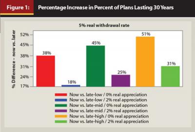
Finally, Figure 1 suggests that the early establishment survival advantage at the 30-year mark over each of the last resort strategies diminishes when higher home appreciation is realized in the future. This phenomenon can be seen through a comparison of the zero and 2 percent real appreciation bars. The rationale behind the estimated reduction in the early establishment survival advantage when higher home appreciation is realized is due to delayed establishment that is based on a future home value that has grown more rapidly since age 62 (or the age for early establishment date) than seen with the lower future home appreciation assumptions. In turn, this leads to a higher line of credit for the last resort scenarios than seen with lower home appreciation.

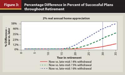
The results shown in Figure 2 and Figure 3 provide a yearly snapshot of the early establishment survival advantage over the last resort establishment strategy where moderate interest rates are experienced at the loan origination date. The early establishment survival advantage represents the percentage increase in early establishment survival rate when compared to the last resort establishment survival rate. Both Figure 2 and Figure 3 are based on a $250,000 home and $500,000 investment portfolio as explained earlier. However, Figure 2 is based on zero percent real annual home appreciation, whereas Figure 3 is based on 2 percent real annual home appreciation.

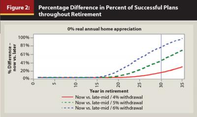
In Figure 2, a 1 percent early establishment survival advantage for the 6 percent real withdrawal rate scenario is estimated to begin at the beginning of year 15 and increase to 77 percent by the end of year 30. Said differently, the early and last resort establishment survival rates for the 6 percent real withdrawal rate scenario are estimated to be 100 versus 99 percent and 67 versus 38 percent at the beginning of year 15 and end of year 30, respectively. For the 5 percent real withdrawal rate scenario, a 1 percent early establishment survival advantage is estimated to begin at the end of year 17 and increase to 45 percent by the end of year 30. Finally, the 4 percent real withdrawal scenario results indicate a 1 percent early establishment survival advantage begins in year 22 of retirement and increases to 14 percent by the end of year 30. 

In Figure 3, a 1 percent early establishment survival advantage for the 6 percent real withdrawal rate scenario is estimated to begin at the beginning of year 16 and increase to 46 percent by the end of year 30. For the 5 percent real withdrawal rate scenario, a 1 percent early establishment survival advantage is estimated to begin at the beginning of year 19 and increase to 25 percent by the end of year 30. Finally, the 4 percent real withdrawal scenario results indicate a 1 percent early establishment survival advantage begins in year 24 of retirement and increases to 6 percent by the end of year 30.⁵

Conclusions

The intent of this study was to outline changes in the HECM program and shed light on two questions; namely, which client-specific and capital market factors should a practitioner emphasize, and based on these various critical factors, how does early or delayed establishment influence whether a reverse mortgage can meet clients’ retirement spending goals? 

The results show an estimated 30-year survival advantage for early establishment. This holds true under various future interest rate and home appreciation scenarios for real withdrawal rates between 4 percent and 6 percent. However, postponing the establishment of an HECM line of credit should be considered when the adviser and/or client has good reason to believe that home occupancy after loan origination is likely to last less than 15 years.

In addition, the results suggest that the 30-year survival advantage associated with early HECM establishment for real annual withdrawal rates at or above 5 percent is estimated to begin between 15 and 20 years after the loan origination date. The advantage could be as high as 85 percent, or 31 percentage points, greater than the last resort survival rates.

The early establishment survival advantage is also shown to exhibit sensitivity to the duration of home occupancy, real withdrawal needs relative to home value, home appreciation, and interest rates. In short, the early establishment survival advantage in today’s interest rate environment is shown to increase with (1) duration of home occupancy, (2) real withdrawal needs relative to home value, (3) higher future interest rates, and (4) lower future home appreciation.

Although it is beyond the scope of this study, it appears that the early establishment survival advantage would also exhibit sensitivity to other factors such as asset allocation, capital market assumptions, taxation, potential future changes to the HECM program, and lending environment. 

Endnotes

1. In 2012, the Consumer Financial Protection Bureau reported that the average lender’s margin ranged from 2.1 percent to 3.0 percent for July 2009 through November 2011. HUD HECM data for loans originated in June 2013 reveal a range of 1.85 percent to 3.25 percent for lender’s margin, with an average of 2.71 percent.
2. Published daily by the Board of Governors of the Federal Reserve System (www.federalreserve.gov/releases/h15/data.htm).
3. Daily data originates from the British Bankers’ Association and is made available by the Federal Reserve Bank of St. Louis (research.stlouisfed.org). 
4. In unreported results, it was determined that a now–high strategy compared less favorably to other scenarios than the now-low strategy. This is because of the lower initial available line of credit when compared to the now-low strategy. For example, a 62-year-old with $250,000 would receive an initial line of credit equal to $105,000 and $46,250, respectively, when established in the now-low versus now-high scenarios. This example assumes all upfront fees are paid from the investment portfolio. Upfront fees of roughly $8,750 represent 8.33 percent and 18.9 percent of initial line of credit in now-low and now-high environments, respectively.
5. A separate analysis was conducted for the same scenarios depicted in Figure 2 and Figure 3 with a beginning investment portfolio value of $250,000, rather than $500,000. It was noted that the early establishment survival advantage over last resort establishment took longer to begin to appear and was smaller than seen with a beginning investment portfolio value of $500,000. These results are available upon request and suggest the potential cost, in terms of a decrease in the likelihood of funding goals, for postponing the establishment of a reverse mortgage decreases as the home value increases, relative to the retirement income needs.

References

AARP. 2011. “Reverse Mortgage Loans: Borrowing against Your Home.” aarp.org. 

Arnott, Robert D., and Peter L. Bernstein. 2002. “What Risk Premium is ‘Normal’?” Financial Analysts Journal 58 (2): 64-85.

Chiuri, Maria C., and Tullio Jappelli. 2010. “Do the Elderly Reduce Housing Equity? An International Comparison.” Journal of Population Economics 23 (2): 643-663.

Consumer Financial Protection Bureau. 2012. “Report to Congress on Reverse Mortgages.” www.consumerfinance.gov.

Cornell, Bradford. 2010. “Economic Growth and Equity Investing.” Financial Analysts Journal 66 (1): 54-64.

Davidoff, Thomas. 2013. “Can ‘High Costs’ Justify Weak Demand for the Home Equity Conversion Mortgage?” SSRN working paper. 

Kitces, Michael E. 2011 (November). “Evaluating Reverse Mortgage Strategies.” The Kitces Report.

Munnell, Alicia H. and Steven A. Sass. 2014. “The Government’s Redesigned Reverse Mortgage Program.” Center for Retirement Research at Boston College.
National Retirement Risk Index. 2010. “Fact Sheet: The NRRI and the House.” Center for Retirment Research at Boston College.

Pfeiffer, Shaun, John R. Salter, and Harold R. Evensky. 2013. “Increasing the Sustainable Withdrawal Rate Using the Standby Reverse Mortgage.” Journal of Financial Planning 26 (12): 55-62.

Sacks, Barry H., and Stephen R. Sacks. 2012. “Reversing the Conventional Wisdom: Using Home Equity to Supplement Retirement Income.” Journal of Financial Planning 25 (2): 43-52.

Salter, John R., Shaun A. Pfeiffer, and Harold R. Evensky. 2012. “Standby Reverse Mortgages: A Risk Management Tool for Retirement Distributions.” Journal of Financial Planning 25 (8): 40-48.

Schulaka, Carly. 2013. “Harold Evensky on ETFs, Reverse Mortgages, and the Most Important Investment in the Coming Decade.” Journal of Financial Planning 26 (6): 16-20.

Sun, Wei, Robert K. Treist, and Anthony Webb. 2007. “Optimal Retirement Asset Decumulation Strategies: The Impact of Housing Wealth.” Public Policy Discussion Paper No. 07-2. Federal Reserve Bank of Boston.

Timmons, J. Douglas, and Ausra Naujokaite. 2011. “Reverse Mortgages: Should the Elderly and U.S. Taxpayers Beware?” Real Estate Issues 36 (1): 46-53.

U.S. Department of Housing and Urban Development. 2013. “Changes to the Home Equity Conversion Mortgage Program Requirements.” HECM Mortgagee Letters. 

Wagner, Gerald C. 2013. “The 6.0 Percent Rule.” Journal of Financial Planning 26 (12): 46-59.

Citation

Pfeiffer, Shaun, C. Angus Schaal, and John Salter. 2014. “HECM Reverse Mortgages: Now or Last Resort?” Journal of Financial Planning 27 (5) 44–51.