Journal of Financial Planning; May 2014
David Blanchett, CFP®, CFA, is head of retirement research at Morningstar Investment Management in Chicago, Illinois. EMAIL AUTHOR.
Executive Summary
- Empirical research on retiree spending has noted a “retirement consumption puzzle,” where retiree expenditures tend to decrease both upon and during retirement. This decrease in spending is inconsistent with general economic theories on consumption, which suggest individuals seek to maintain constant consumption over their lifetimes.
- Government data on consumption was analyzed in this study to understand how retiree consumption actually changes over time.
- The results of the analysis suggest that although the retiree consumption basket is likely to increase at a rate that is faster than general inflation, actual retiree spending tends to decline in retirement in real terms. This decrease in real consumption averages approximately 1 percent per year during retirement.
- A “retirement spending smile” effect is noted. This finding has important implications when estimating retirement withdrawal rates and determining optimal spending strategies.
Acknowledgement: The author thanks Alexa Auerbach and Hal Ratner for helpful edits and comments.
Retirement income research and financial planning tools generally assume that retiree expenditures, or consumption, increase annually by inflation during retirement. This assumption is counter to a growing body of empirical research that has noted actual retiree expenditures tend to decrease both upon, and during, retirement. This phenomenon has been named the “retirement consumption puzzle.
Decreased inflation-adjusted spending is inconsistent with general economic theories on consumption, such as the life-cycle hypothesis, which suggests individuals seek to maintain constant consumption over their lifetimes. Decreased inflation-adjusted spending also conflicts with assumptions underlying the majority of retirement income research that assume retirement income should increase annually by inflation.
For this paper, government data on consumption was analyzed to understand how retiree consumption actually changes over time. The results of the analysis suggests that although the retiree consumption basket is likely to increase at a rate that is faster than general inflation—a fact that can largely be attributed to the higher weight to medical expenses for retirees—actual retiree spending tends to decline in retirement in real terms. This decrease in real consumption averages approximately 1 percent per year during retirement.
A “retirement spending smile” effect is noted. Changes in real consumption tend to be greater in both early and late retirement. This means that although the basket of goods consumed by retirees may increase faster than total inflation, total spending actually decreases.
Literature Review
A growing body of literature explores the spending habits and tendencies of retiree households. The majority of these studies note that inflation-adjusted consumption tends to decline at and during retirement. This decrease in real spending is counter to various economic theories on consumption, such as the life-cycle hypothesis (LCH), as well as common assumptions used in retirement income research.
The LCH was introduced by Modigliani and Brumberg (1954) and implies that individuals maximize utility by planning savings and consumption such that lifetime consumption is as smooth as possible. Financial planning tools and retirement income research often take an LCH perspective on spending and generally assume that retiree expenditures increase annually by inflation.
Changes in retiree consumption vary by study. Banks, Blundell, and Tanner (1998) were perhaps the first to note a sharp decline in consumption at retirement. Banks et al. used U.K. data. Using panel data from the Panel Study of Income Dynamics (PSID), Bernheim, Skinner, and Weinberg (2001) noted a similar effect. Also using panel data, Hurd and Rohwedder (2008) found that spending before and after retirement declines at a relatively small rate, from 1 percent to 6 percent depending on the measure. Research by Aguila, Attanasio, and Meghir (2011) noted that individuals tend to smooth consumption during the first year of retirement.
Ameriks, Caplin, and Leahy (2007) analyzed responses to survey questions answered by TIAA-CREF participants about anticipated changes in spending at retirement among those still working and about recollected spending changes among those who were already retired. They found that the mean anticipated change was –11.3 percent versus the recollected change of –4.6 percent. They also found that 54.6 percent of their sample anticipated a reduction in spending, versus 36.2 percent that recollected a reduction. This suggests the actual reduction in spending for retirees may be less than many forecast.
These findings are similar to results reported by others, including Miniaci, Monfardini, and Weber (2003) and Battistin, Brugiavini, Rettore, and Weber (2007) who used the Italian Survey on Family Budgets, as well as Aguiar and Hurst (2008) and Laitner and Silverman (2005) who used the Consumer Expenditure Survey.
In particular, Fisher, Johnson, Marchand, Smeeding, and Torrey (2008) found that consumption expenditures decrease by about 2.5 percent when individuals retire; expenditures continue to decline at about a rate of 1 percent per year after that. In contrast, Christensen (2004), using Spanish panel data, found no evidence of a drop in consumption at retirement in any of the commodity groups analyzed.
The change in expenditures varies by expenditure type, although there is a growing body of research focusing solely on food expenditures. Aguiar and Hurst (2005) noted that although food expenditures decline 17 percent at retirement, the quantity and quality of food consumed does not change. In contrast, Haider and Stephens (2007) found in the PSID and in the Retirement History Survey that people reduce spending on food when they retire by about 5 percent to 10 percent. Using panel data from 1980 through 2000, Aguila, Attanasio, and Meghir (2011) estimated a 6 percent drop in food expenditures after retirement, although they found no evidence of non-durable spending reduction in other areas. They attributed this decline in food expenditures to the additional time retiree households have to produce food at home and shop for bargains.
Hurst (2008) surveyed the existing literature and noted there may not be a retirement consumption puzzle after all. He noted that declines in expenditures, aside from work-related expenses, primarily occur in food; furthermore, the declines are largest for those who involuntarily retire. Therefore, a lifecycle consumption augmented with home production and uncertain health shocks does a relatively good job of explaining the consumption patterns of most households as they transition into retirement. These varied perspectives are tested in this paper.
Retiree Expenditures
The basket of goods and services consumed by individuals is not constant over time. Expenses, such as medical costs, generally increase as a percentage of total expenditures as someone ages. To better understand how spending changes over time, data from the 2011 Consumer Expenditure Survey (CEX) was explored. The CEX provides information on the buying habits of American consumers and is collected for the Bureau of Labor Statistics by the U.S. Census Bureau. The CEX is used by various groups, perhaps most importantly to regularly revise the Consumer Price Index (CPI), which is in the most common metric for general inflation.
For the analysis, spending was grouped by household age, which is either the age of the reference person for a single household or the average of the reference person and the spouse for a two-person household. Values for the primary expenditure categories were reviewed to estimate total expenditures (code TOTEXPPQ). Spending on the following individual categories was obtained: clothing (APPARPQ), charitable contributions (CASHCOPQ), food (FOODPQ), entertainment (ENTERTPQ), health care (HEALTHPQ), housing (HOUSPQ), insurance and pensions (PERINSPQ), and transportation (TRANSPQ). The remainder of consumption was combined into a single “other” category.1 Average expenditures for the nine different categories were averaged by age, from age 25 to age 85, as shown in Figure 1.
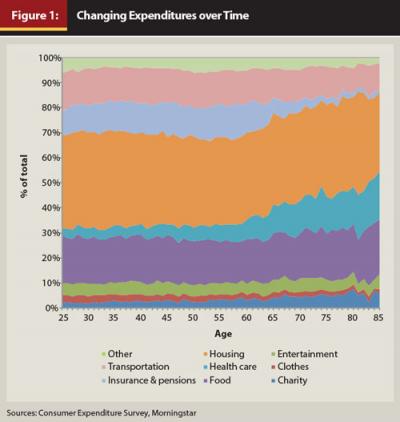
Two notable changes in average consumption occur as households age: the relative amount spent on insurance and pensions decreases significantly at older ages, and the relative amount spent on health care increases significantly at older ages. Medical care expenses represent approximately 10 percent of total expenditures for a 65-year-old household, but increase to approximately 20 percent by age 85.
Varying consumption profiles have important implications when estimating the levels of expected inflation for different individuals. The most common measure of inflation is based on changes in CPI for urban consumers, or the CPI-U. Alternative versions of the CPI exist to reflect the varying consumption baskets of different types of households. For example, the CPI for urban wage earners and clerical workers (CPI-W) is used to determine the increase in Social Security benefits. However, the CPI-U is generally accepted to be a better definition of aggregate inflation, because it encompasses 87 percent of the population, versus only 32 percent of the population for the CPI-W.
A specific CPI version created for retirees, or more specifically for the elderly, is called the Experimental CPI for Americans 62 Years of Age and Older, which is more commonly referred to as the CPI for the elderly (CPI-E). Table 1 contrasts the differences in the relative weights for different expenditures between the CPI-U, CPI-W, and CPI-E.
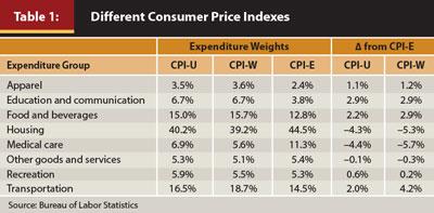
The CPI-U and CPI-W are relatively similar, however there are notable differences in the CPI-E. One of the biggest differences is the higher weight to medical expenses in the CPI-E. The weights in Table 1 suggest that older individuals tend to devote a higher percentage of total expenditures to medical care expenses; they also tend to spend less on things such as education, apparel, and transportation. This pattern of spending is consistent with general theoretical expectations.
The average historical annual change in the CPI-E from December 1982 to December 2012 was 3.07 percent versus 2.92 percent for the CPI-U. In other words, the rate of inflation for retiree expenditures has increased at a faster rate than general inflation. A key reason why CPI-E has increased at a faster rate than CPI-U, and is likely to continue doing so, is the high historical rate of medical care inflation compared to general inflation. Medical care inflation, defined as the change in CPI for All Urban Consumers: Medical Care,2 has increased at a rate that is approximately 50 percent faster than general inflation from 1948 through 2012 (5.42 percent and 3.63 percent, respectively). Current projections for future increases in medical costs exceed 7 percent per year.
Given the higher weight of medical expenses for retirees, and the fact medical expenses have historically increased at a rate faster than inflation, and are generally projected to continue doing so, it is likely that retiree expenses will increase at a rate that is faster than inflation. This suggests that models that use general inflation measures to forecast the change in retirement expenditures are likely underestimating the amount of savings required to fund retirement. However, just because the expenditure basket for retirees is projected to increase at a rate that is higher than general inflation does not mean retiree expenditures will actually increase by an amount greater than inflation. This concept will be explored in the next section.
Retiree Spending
In the previous section, the differences in consumption profiles for households of different ages were explored. In this section, the actual changes in total consumption (or expenditures) for retiree households over time are reviewed. Reviewing actual expenditures is important because it provides insight as to whether retiree spending does in fact increase annually by inflation—a common assumption. This analysis is especially relevant given the findings of the previous section, which suggest retiree spending should increase by a rate that is faster than inflation, given the higher weight of medical expenditures for retirees.
The RAND Health and Retirement Study (HRS) dataset was used to determine actual changes in consumption for retirees. The HRS is a panel household survey that combines both cross-sectional and longitudinal data. The HRS is specifically focused on the study of retirement and health among individuals over the age of 50 living in the United States.3
For the analysis, RAND HRS spending data was matched to RAND Consumption and Activities Mail Survey (CAMS) data for each household. While the RAND HRS data has detailed information about household attributes, the RAND CAMS data provides detailed information about household spending. The CAMS survey was first mailed in September 2001 and has been sent every two years since. For the analysis, each of the five available RAND CAMS series from 2001 through 2009 was reviewed and matched to the appropriate RAND HRS dataset.
A number of filters were applied to the available household data:
- Consumption data for the household needed to be available for each of the surveys in order to be included.
- The household must have considered itself retired.
- The total consumption of the household must have exceeded $10,000 for each of the five surveys.
- The maximum potential consumption change could not be greater than 50 percent, in absolute terms, between any two of the five surveys.
These filters reduced the test sample to 591 households, which is 10.9 percent of the total number of households available in the CAMS series.
Real growth in consumption was estimated by reducing the actual change in consumption by the increase in the CPI-U over the respective period between each of the surveys. After the average annual real change for each household was estimated for each age, the average change for all households that age was used to represent the change in real consumption for that age group. Similar to the aggregation methodology for the CEX data, the age for a single household was based on the age of that household individual, while the age for married household was the average age of the two spouses.
Figure 2 includes the annual inflation-adjusted change in consumption for retirees from age 60 to age 90. The results are bounded by these ages to ensure a large enough sample of retirees at each age (approximately 30 households by age). A second order polynomial regression was performed for the entire age range, as well as from ages 65 to 75. The smaller age range regression (age 65 to 75) is included in Figure 2, because future tests are limited to that range for sample size reasons.
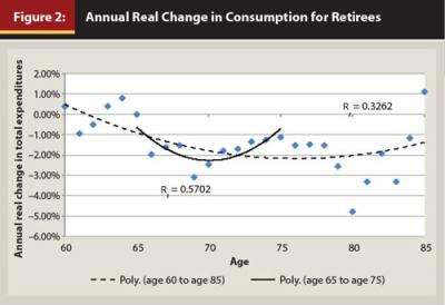
The results of this analysis are consistent with past research. Retiree expenditures decrease during retirement. This supports the notion that the retirement consumption puzzle exists. For example, Bernicke (2005) noted that older households tend to spend less than younger households. Research by Banerjee (2012) also noted a similar effect. The average real change in retiree spending in this study from age 60 to age 90 was –0.96 percent per year, with a statistically significant t statistic of –4.31.
The actual changes in real retirement spending create a “retirement spending smile” whereby the expenditures increase at a faster rate (although these are still negative) for relatively younger and relatively older retirees. The “smile” can likely be attributed to the fact younger retirees are better able to travel and enjoy retirement, while older retirees incur higher relative medical expenses. The overall changes in real spending, though, are clearly negative; the only real variation is the extent of the negative change.
By Choice or By Need?
The changes in spending noted in Figure 2 clearly suggest retiree spending decreases, in real terms, over time. What is less clear, though, is whether the reduction in expenditures is by choice or by need. It may be that retirees have under saved, on average, and are forced to reduce consumption to avoid retirement ruin. This would be consistent with how retirement savings are generally portrayed in the media. Although it is impossible to entirely disentangle this effect, an additional analysis was performed where the households were placed in four groups based on the amount of consumption and household net worth. For both categories, the “cut off” to separate the low and high groups was based on the approximate median values over the entire period of available data, which is an annual consumption of $30,000 and a total net worth of $400,000.
The net worth definition includes the value of financial and nonfinancial assets. Additionally, the value of pensions and Social Security retirement benefits were included and estimated by calculating the mortality-weighted net present value of the future benefit payments. A discount rate of 2 percent was used when estimating the value of Social Security retirement benefits. A discount rate of 4 percent was used for pensions, which were assumed to be nominal. Life probabilities were based on the unisex mortality rates from the Society of Actuaries 2000 Annuity Table.
Four household groups were created for the analysis. Households with below-average consumption and below-average net worth were labeled “low spend, low net worth.” Households with average consumption and average net worth were labeled “high spend, high net worth” households. Along these same lines, the remaining two groups were categorized “low spend, high net worth” and “high spend, low net worth."
Categorizing households into these four groups allows for a better understanding of how consumption varies. Households that have “matched” levels of spending and net worth (low/low and high/high), are assumed to be consuming optimally—that is, their consumption is roughly consistent with resources. In contrast, households where spending and net worth are not the same (high/low or low/high), are consuming sub-optimally, either too much (high/low) or not enough (low/high).
The real changes in consumption over time for these four groups are contrasted in Figure 3, where Panel A is the matched households and Panel B is the mismatched households.
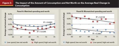
The “matched” groups in Panel A of Figure 3 have relatively similar average real changes in expenditures from ages 65 to 75. However, lower spending households tend to have lower decreases in spending over time. This can potentially be attributed to the fact households with higher levels of consumption may spend more on nondiscretionary items, and that spending decreases at a faster rate as the individual ages.
There is a much greater difference in the change in real spending for the mismatched households (Panel B of Figure 3). Households that are overfunded and not spending optimally (the “low spend, high net worth” group) actually tend to increase consumption as they move from age 65 to age 75, but at a decreasing rate. Even though a low spend, high net worth household could potentially increase consumption, it continues to decline at higher ages. In contrast, those households that are underfunded and spending too much tend to see considerable declines in consumption; this could be brought on by the realization that household spending is not sustainable.
Modeling the Impact
An analysis was performed to provide insights into how the previous findings could affect retirement income modeling, and as a result, optimal retirement income strategies.
For the analysis, changes in real retiree annual spending (ΔAS) was estimated using equation 1, where the change was estimated as a function of age (Age) and after-tax total expenditures (ExpTar) of the retiree. Equation 1 was determined using results from the previous analysis, as well as additional regressions; the formula was adjusted slightly so that increases in spending are higher than noted by historical data. This subjective change was made to account for future potential increases in medical care costs and to potentially correct for reductions in retiree consumption that are brought on by lack of savings.
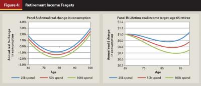
ΔAS = .00008(Age2) – (.0125 * Age) – .00661n(ExpTar) + 54.6% [1]
Three different “spending curves” were estimated using equation 1. As shown in Figure 4, each was based on three different initial target retirement spending goals: $25,000, $50,000, and $100,000, respectively. The resulting change in annual spending by age is included in Panel A. The annual real income withdrawal goal for a 65-year-old retiree is included in Panel B. The most common assumption with respect to retiree expenditures is that expenses increase with inflation. If included in Panel A, this would be a horizontal line at the 0 percent mark and a horizontal line at the $1 mark in Panel B.
To determine the impact of different retirement spending curves on the cost of retirement, a Monte Carlo analysis was performed. For the first batch of scenarios, the probability of a withdrawal strategy lasting over a 30-year retirement period was determined based on a constant real spending need, as well as the $25,000, $50,000, and $100,000 spending curves. The term “initial withdrawal rate” is used here to note the initial amount withdrawn from the portfolio, where the amount is changed by some amount going forward. The constant real spending curve assumes the need increases annually by inflation, while changes in the withdrawal amount of the spending curves was determined using equation 1.
Each test scenario was based on a 10,000-run Monte Carlo simulation that was assumed to last 30 years. The analysis assumed retirement assets are invested in a portfolio that is allocated 40 percent to stocks and 60 percent to bonds. The portfolio was assumed to have a real return of 3 percent and a standard deviation of 10 percent. These portfolio assumptions were based approximately on Ibbotson’s 2013 capital market estimates. Taxes were ignored for the analysis, as are any type of required minimum distributions.
Initial withdrawal rates from 2 percent to 8 percent were tested in 0.2 percent increments. It is important to note that a 4 percent initial withdrawal rate would result in the same withdrawal from the portfolio; the ongoing withdrawal will vary depending on how the assumed need changes over time (see the spending curves in Figure 4). Results from the Monte Carlo simulations are included in Figure 5.
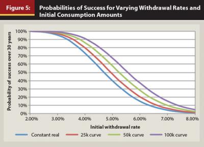
The probabilities of success increase across the different initial withdrawal rates when using the spending curves versus assuming an increase in constant real withdrawal amounts. This is not surprising, because the spending curves effectively assume lower future withdrawals from the portfolio. For example, a 4 percent initial withdrawal rate has a 73.3 percent probability of success using a constant real strategy (where the withdrawal increases each year by inflation), while the 25,000 curve has a 79.9 percent chance of success, the 50,000 curve has an 86.0 percent, and the 100,000 curve a 91.1 percent.
Mortality was incorporated in the second batch of scenarios. Although a fixed retirement period (for example, 30 years) is a simplifying assumption commonly used in retirement income research, it does not reflect the possibility of true failure for a retiree. A portfolio has only truly failed when it can no longer sustain the target withdrawal amount while one (or both) member(s) of the household is (are) still living. The differences between modeling for a fixed period (assuming a death date) and modeling for conditional mortality were noted by Blanchett and Blanchett (2008).
For the mortality scenarios, the definition of success was changed from being able to generate the target amount of income for a 30-year period to generating income while at least one member of the household is still living. Three households were considered: a male age 65, a female age 65, and a married couple (male and female, both age 65). Mortality was based on the Society of Actuaries 2000 Annuity Table. Fixed retirement periods of 20, 25, 30, 35, and 40 years were also included for comparison purposes. Results are shown in Table 2.
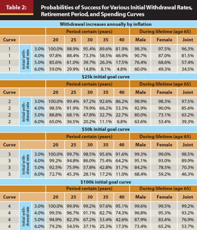
Table 2 provides information about the probability of success for different initial withdrawal rates over varying retirement periods. Four different withdrawal rate assumptions were used (similar to Figure 5), where the withdrawal amount was increased annually by inflation or changes were based on the initial spending goal ($25,000, $50,000, or $100,000) using equation 1. A successful outcome was defined as the portfolio providing income for the duration of retirement, which is either a fixed period (for example, 30 years) or based on the lifetime of the retiree (male, female, or joint couple).
The results shown in Table 2 suggest that the relative safety of a withdrawal strategy varies materially based on the assumed spending curve and the retirement period (either the number of assumed years or a life expectancy model). Using the constant real model, a 4 percent initial withdrawal rate has a 73.3 percent probability of success over a 30-year period. The probability of success for a 4 percent initial withdrawal rate using the constant real model increases to 81.5 percent over the expected mortality of a joint couple (male and female both age 65).
Moreover, the success rate for the joint couple climbs even higher to 89.9 percent if one assumes a $50,000 spending curve rather than a constant real model. Another way of looking at the results is that the 4 percent initial withdrawal scenario over 30 years under the constant real model has the same approximate probability of success (70.3 percent versus 73.3 percent) as the 5 percent initial withdrawal scenario with the $50,000 spending curve over the expected mortality of the couple.
A 5 percent initial withdrawal rate results in a 20 percent reduction in the amount of savings required to fund a retirement goal when compared to a traditional 4 percent initial withdrawal rate. This may seem counter intuitive, but if it is assumed that a retiree household requires $40,000 of income per year from a portfolio, using the 5 percent rule, the necessary balance at retirement is $800,000 ($40,000/0.05 = $800,000) versus $1 million if a 4 percent initial withdrawal rate is used. This 5 percent initial withdrawal amount can likely be further increased if the retiree is willing to take on the potential risk of future reductions in spending by implementing a more dynamic withdrawal strategy.
Implications
The analysis conducted for this paper has a number of important implications for financial planners and their retiree clients. First, it may be that many retirement modeling tools are overestimating the cost of retirement. Empirical data on actual retiree spending suggests that retiree consumption does not increase annually by inflation. While it is difficult to determine whether this real reduction is due to a lack of retirement resources or active choice (or some combination of the two), the “retirement consumption puzzle” appears to be a very real phenomenon.
The fact that spending tends to decrease in real terms during retirement may lead to suboptimal retirement consumption. Retirees may be better served by planning on spending more early in retirement (and saving more for later in retirement) than assuming some constant inflation-adjusted amount. Spending more early in retirement also allows retirees the ability to spend money on things they may be unable to enjoy later in retirement as health declines.
Reductions in real spending also have important implications for optimal guaranteed income. Inflation-adjusted single premium immediate annuities (SPIAs) are often noted as “risk-free” retirement income assets, because they hedge both inflation risk and mortality risk. If retiree spending does not increase annually by inflation, though, it may be that some combination of a nominal annuity and inflation-adjusted annuity would be a more optimal combination of guaranteed income. This possibility is worthy of future study. Finally, gaining a better appreciation of how future medical care expenses will affect retirees is of importance. This is an essential issue that is difficult to model. Medical care expenses clearly represent an increasing portion of retiree expenditures over time; as such, future relative increases could increase the relative weight.
Conclusions
The purpose of this paper was to explore retiree spending, along with the well-documented “retirement consumption puzzle,” an effect noted in past research where consumption tends to decrease in inflation-adjusted terms upon and during retirement. Data on consumption baskets suggests that retiree spending should likely increase at a rate that is faster than general inflation, given the higher weight of medical care expenses for retirees and the higher historical inflation rate associated with these expenses. However, in this study, actual retiree expenditures did not show a positive linear pattern. Rather, a “retirement spending smile” was noted with respect to changes in real spending overtime, where overall change in real spending was negative (approximately –1 percent per year during retirement, on average), although higher during both early and late retirement.
These findings are contrary to key general economic theories on consumption, such as the life-cycle hypothesis, which suggests individuals seek to maintain constant consumption over their lifetimes. Results also conflict with assumptions underlying the majority of retirement income research, which assume retirement income should increase annually by inflation. Findings from this study also have important implications for financial planners when estimating retirement withdrawal rates and determining optimal spending strategies. In summary, it appears that a more nuanced perspective of retiree expenditures can potentially yield a better estimate of the true cost of retirement.
Endnotes
- Alcoholic beverages (ALCBEVPQ), personal care (PERSCAPQ), reading (READPQ), education (EDUCAPQ), and tobacco (TOBACCPQ).
- Data obtained from the Federal Reserve Bank of St. Louis (FRED).
- The RAND HRS is a user-friendly version of a subset of the HRS that contains cleaned and processed variables with consistent and intuitive naming conventions, model-based imputations and imputation flags, and spousal counterparts of most individual level variables.
References
Aguiar, Mark, and Erik Hurst. 2005. “Consumption vs. Expenditure.” Journal of Political Economy 113 (5): 919–948.
Aguiar, Mark, and Erik Hurst. 2008. “Deconstructing Lifecycle Expenditure.” National Bureau of Economic Research Working Paper No. w13893.
Aguila, Emma, Orazio Attanasio, and Costas Meghir. 2011. “Changes in Consumption at Retirement: Evidence from Panel Data.” Review of Economics and Statistics 93 (3): 1094–1099.
Ameriks, John, Andrew Caplin, and John Leahy. 2007. “Retirement Consumption: Insights from a Survey.” Review of Economics and Statistics 89 (2): 265–274.
Banerjee, Sudipto. 2012. “Expenditure Patterns of Older Americans, 2001–2009.” EBRI Issue Brief (February).
Banks, James, Richard Blundell, and Sarah Tanner. 1998. “Is there a Retirement-Savings Puzzle?” American Economic Review 88 (4): 769–788.
Battistin, Erich, Agar Brugiavini, Enrico Rettore, and Guglielmo Weber. 2007. “The Retirement Consumption Puzzle: Evidence from a Regression Discontinuity Approach.” University Ca’Foscari of Venice, Dept. of Economics Research Paper Series 27/07.
Bernheim, B. Douglas, Jonathan Skinner, and Steven Weinberg. 2001. “What Accounts for the Variation in Retirement Wealth Among U.S. Households?” American Economic Review 91 (4): 832–857.
Bernicke, Ty. 2005. “Reality Retirement Planning: A New Paradigm for an Old Science.” Journal of Financial Planning 18 (6): 56–61.
Blanchett, David M., and Brian C. Blanchett. 2008. “Joint Life Expectancy and the Retirement Distribution Period.” Journal of Financial Planning 21 (12): 54–60.
Christensen, Mette. 2004. “Demand Patterns around Retirement: Evidence from Spanish Panel Data.” Economics Discussion Paper Series EDP-0809.
Fisher, Jonathan D., David S. Johnson, Joseph Marchand, Timothy M. Smeeding, and Barbara Boyle Torrey. 2008. “The Retirement Consumption Conundrum: Evidence from a Consumption Survey.” Economics Letters 99 (3): 482–485.
Haider, Steven J., and Mel Stephens. 2007. “Is There a Retirement-Consumption Puzzle? Evidence Using Subjective Retirement Expectations.” Review of Economics and Statistics 89 (2): 247–264.
Hurd, Michael D., and Susann Rohwedder. 2008. “The Retirement Consumption Puzzle: Actual Spending Change in Panel Data.” National Bureau of Economic Research Working Paper No. w13929.
Hurst, Erik. 2008. “The Retirement of a Consumption Puzzle.” National Bureau of Economic Research Working Paper No. 13789.
Laitner, John, and Dan Silverman. 2005. “Estimating Life-Cycle Parameters from Consumption Behavior at Retirement.” National Bureau of Economic Research Working Paper No. 11163.
Miniaci, Raffaele, Chiara Monfardini, and Guglielmo Weber. 2003. “Is There a Retirement Consumption Puzzle in Italy?” Institute for Fiscal Studies Working Paper No. 03/14.
Modigliani, Franco, and Richard Brumberg. 1954. “Utility Analysis and the Consumption Function: An Interpretation of Cross-Section Data.” In Post-Keynesian Economics, edited by Kenneth K. Kurihara. New Brunswick, NJ: Rutgers University Press.
Citation
Blanchett, David. 2014. “Exploring the Retirement Consumption Puzzle.” Journal of Financial Planning 27 (5): 34–42.