Journal of Financial Planning: May 2013
Executive Summary
- Past research has introduced the concept of “Gamma,” which is a metric designed to quantify the potential retirement income benefits that an investor can realize from making intelligent financial planning decisions.
- This paper continues this line of research, but focuses on the accumulation phase, examining the relative importance of four different factors called the “ABCDs of Retirement Success.” These factors are: Alpha, Beta, Cash Flows (savings for accumulators and distributions for retirees), and the benefits of Delayed Retirement.
- Through multivariate regressions and constrained optimizations, this research shows the relative importance of each factor for different scenarios. We find that while each of the different factors considered are important, they are not equally important, and affect outcomes differently.
- For example, the relative importance of Cash Flows depends on the size of an investor’s account balance. We also find that for a hypothetical investor nearing retirement, delaying retirement a single year can increase the probability of success by approximately 10.6 percent, which is approximately equivalent to generating 1.0 percent of Alpha during each year of the entire retirement period.
David M. Blanchett, CFP®, CLU®, AIFA®, CFA, (david.blanchett@morningstar.com), is the head of retirement research for Morningstar Investment Management, in Chicago, Illinois.
What drives successful outcomes for individual investors? The financial advisory community has primarily focused on concepts like Alpha and Beta, yet these concepts only represent one part of an individual investor’s financial plan: the investment part. Past research by Blanchett and Kaplan (2012) introduced the concept of “Gamma,” which is a metric designed to quantify the potential benefits that an investor can realize from making intelligent financial planning decisions. This paper continues that line of research with a focus on quantifying the relative importance of four concepts called the “ABCDs of Retirement Success.” These factors are: Alpha, Beta, Cash Flows (savings for accumulators and distributions for retirees), and the benefits of Delayed Retirement.
Through multivariate regressions and constrained optimizations, this paper illustrates the relative importance of each factor under different scenarios. While each of the factors is important, they are not equally important, with each factor affecting outcomes differently. For example, the relative importance of Cash Flows depends on the size of an investor’s account balance. We also find that for a hypothetical investor nearing retirement, delaying retirement a single year can increase the probability of success by approximately 10.6 percent, which is approximately equivalent to generating 1.0 percent of Alpha during each year of the entire retirement period. This research has important implications for a variety of readers, most specifically financial planners, 401(k) plan sponsors, and individual investors.
A Review of Alpha and Beta
There are easily hundreds, if not thousands, of research papers devoted to exploring Alpha and Beta. Alpha and Beta are concepts related to investing, and within the context of this paper, Beta is defined as the market asset allocation, or exposures, of a portfolio, while Alpha is the residual component of the portfolio return that cannot be attributed to the market asset allocation (that is, Beta). For example, if a client’s portfolio returns 8 percent, and the Beta-relevant (that is, factor-adjusted) portion of the portfolio returns 10 percent, the Alpha, or the residual return not explained by the Beta factors, would be −2 percent (8 percent less 10 percent = −2 percent). The Alpha is driven by a variety of factors, such as fees (which negatively affect Alpha) or skills (which can positively or negatively affect Alpha).
The importance of an adviser’s ability to generate Alpha and Beta for an investor depends on the engagement. If the financial adviser’s sole responsibility is to manage a portfolio of assets without offering any additional services, such as financial planning advice, Alpha and Beta should be relatively good metrics to quantify the value created by the adviser. In more complex engagements (for example, when financial planning services are being provided), value cannot be defined by Alpha and Beta alone. This is because within a financial planning context the objective is usually to achieve a goal, not just a return, and Alpha or Beta are merely two of the many variables associated with achieving that goal.
A financial adviser could generate negative Alpha for a client (for example, through poor mutual fund selection) but still provide other valuable services that enable a client to achieve his or her goals (for example, retire). While the negative Alpha may have required the client to save more for retirement, the underlying goal was still accomplished. The financial planning services could have more than offset the “cost” associated with the negative Alpha. Therefore, it is possible to lose the Alpha (and Beta) battle, but win the war (that is, retirement success) through intelligent financial planning.
And Now Gamma …
Gamma, which is the third letter in the Greek alphabet, preceded by Alpha and Beta, is a metric introduced by Blanchett and Kaplan (2012), BK herein, to measure the potential benefits an investor can achieve by making intelligent financial planning decisions. This is a concept Bennyhoff and Kinniry (2010) called “advisor’s alpha” and Scott (2012) called “household alpha.” In their initial research on the topic, BK focused on five fundamental financial planning techniques for retirees: (1) a total wealth framework to determine the optimal asset allocation, (2) a dynamic withdrawal strategy, (3) incorporating guaranteed income products (that is, annuities), (4) tax-efficient decisions, and (5) liability-relative asset allocation optimization. These five factors are by no means an exclusive list of the value that can be realized from quality financial planning.
BK found that following a “Gamma-optimized” approach for the five techniques considered can yield 28.8 percent more income for a hypothetical retiree on a utility-adjusted basis when compared to a naïve, base case portfolio. This 28.8 percent in additional income during retirement is equivalent to achieving a return increase (that is, annual Alpha) of 1.82 percent for each year during retirement. Creating 1.82 percent in Alpha for a client for the entire retirement period would likely be considered a significant achievement, although in this case, simulations demonstrated these results can be achieved by efficient financial planning.
The central concept behind Gamma is that the decisions a financial planner makes can add significant value beyond just investment manager selection (Alpha) and asset allocation (Beta). While these benefits may be difficult to quantify, they are very real and can significantly affect an investor’s outcome. This paper takes a more holistic approach to quantifying the decisions that affect better outcomes for a client by focusing on the relative importance of Alpha, Beta, Cash Flows, and Delayed Retirement. Understanding the relative importance of the factors that drive retirement outcomes can enable an adviser to focus on what matters and better help a client achieve his or her goals.
The analyses seek to determine the relative importance of Alpha, Beta, Cash Flows, and Delayed Retirement using various tests, primarily through deterministic and stochastic modeling coupled with multivariate and constrained regressions.1 This approach allows for modeling different outcomes and then determining the relative impact each factor has based on the regression coefficients (that is, the factors of retirement success). Regression coefficients are commonly referred to as “betas,” however, to remove any potential confusion with the Beta notation used in this article, which refers to the market exposure of a portfolio, the term “regression coefficient” is used to describe the relationship between the dependent and independent variables in the regression.
Three primary scenarios are reviewed. The first scenario explores the relative importance of Alpha, Beta, and Cash Flows to account balance growth for someone who is currently in the accumulation phase. The second scenario reviews the relative importance of Alpha, Beta, and Cash Flows to achieving the retirement goal as measured by the probability of success. The third scenario adds the potential impact of Delayed Retirement to Alpha, Beta, and Cash Flows as it relates to achieving retirement success. This paper is similar in scope to Blanchett and Grantz (2011) who calculated the “drivers of retirement success,” although the tests for this analysis are more complex, considering both accumulation and retirement and introducing new factors.
Accumulation Analysis
The first analysis looks at the relative impact of Alpha, Beta, and Cash Flows to the growth of a portfolio over a year. The impact is determined by running deterministic scenarios and regressing the Alpha, Beta, and Cash Flow inputs used for the calculations on the results of the time value of money calculations. The regressions, therefore, demonstrate the impact each component has on the growth of the hypothetical account balance of the portfolio at the end of the year.
For the analysis, 125 scenarios were considered: five Alpha scenarios (alpha from −2 percent to 2 percent, in 1-percent increments), five Beta scenarios (equity allocations from 0 percent to 100 percent in 25-percent increments), and five Cash Flow scenarios (savings from 0 percent to 12 percent in 3-percent increments). We assume a 10 percent annual return for stocks with a 20 percent standard deviation, a 4 percent annual return for bonds with a 7 percent standard deviation, and a correlation of 0.1 beween stocks and bonds. We assume an annual inflation rate of 2.5 percent. These values are the approximate 20-year Ibbotson Capital Market Forecasts as of June 2012. While different equity allocations are tested, the compounded nominal return is the dependent variable used in the regression. This allows the Beta regression coefficient to be more easily compared to Alpha in terms of its relative importance.
The annual compensation for the hypothetical worker is assumed to be $100,000. Therefore, a savings rate of 9 percent would yield a total savings amount of $9,000 ($100,000 ≈ 9% = $9,000). All savings are assumed to take place at the end of the year. The relative importance of the three components will vary based on the size of the portfolio. The greater the portfolio balance the more we would expect Alpha and Beta to affect the variation in the change in portfolio value over the year versus the Cash Flows. The portfolio size is proxied as the ratio of the account balance to annual income. Under this framework, given an assumed income of $100,000, a balance-to-income ratio of 5 would suggest an account balance of $500,000. This framework enables the reader to compare the respective impact regardless of income, as these estimates can be used for someone making $30,000 or $300,000, for example.
The regressions for each calculation are simple multivariate regressions, where the independent variable (for example, the growth in an account value for the accumulation scenario) is regressed against different Alpha, Beta, and Cash Flow values. We do not set the intercept to zero or run a constrained regression for the analysis. We vary the Alpha, Beta, and Cash Flow values (in the case for the accumulation scenario across the 125 potential inputs) to determine the relative importance of each dependent variable.
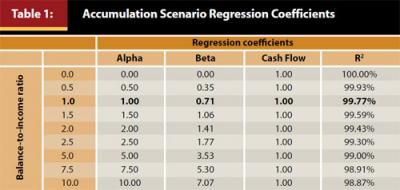
The resulting regression coefficients for the 125 simulations are included in Table 1. It is important to note that the results are in some ways redundant as the Alpha and Beta regression coefficients are scalable based on the size of the portfolio while the Cash Flow regression coefficient is constant. For example, the regression coefficients for Alpha and Beta for the 10.0 balance-to-income ratio are 10 times the regression coefficients when compared to the 1.0 balance-to-income ratio test. The different regression coefficients at each balance-to-income ratio are included for informational purposes for the reader.
For Table 1, the nominal return used for the Beta regression coefficients is the compounded nominal return of the portfolio versus the simple arithmetic return. Over a one-year period the simple arithmetic return is a better estimate of the outcome than the compounded return, but the compounded return is used to make this analysis more consistent with later tests that use a simulation approach and therefore implicitly considers the variance drain. Variance drain is a term used to describe the fact that negative returns have a greater impact on the realized return than positive returns. For example, if an investor achieves a return of +100 percent in one year and −50 percent the next while the arithmetic average return is +25 percent the geometric average, or the return actually realized by the investor over the two-year period, is 0 percent.
The variance drain reduction in Beta is important because the long-term incremental benefit of Alpha is greater than Beta, because there is no variance drain with Alpha return, as there is with Beta return. Investors who seek to potentially increase their returns by increasing the equity allocation do so at the peril of higher market risk (that is, portfolio standard deviation), which reduces the eventual compounded return achieved by the investor.
For readers not familiar with interrupting regression coefficients, within the context of Table 1, they represent the percentage change in the account balance (in dollars) over the next year given a 1 percent change in any of the variables—Alpha, Beta, or Cash Flows. For example, under the balance-to-income ratio of 1.0 scenario, a 1 percent increase in the Alpha return would lead to a 1 percent increase in the balance during the year (1.00 ≈ 1% = 1%), a 1 percent increase in the Beta return would increase the balance by only 0.71 percent (0.71 ≈ 1% = 0.71%). The reason a 1 percent increase in Beta is less than the Alpha increase is due to the variance drain associated with investing in a more aggressive market portfolio. In contrast, Alpha is a “risk-free,” or residual, positive or negative return. Both Beta and Alpha are assumed to be constants throughout the simulation period.
The constant regression coefficient for Cash Flows (1.00) may also surprise the reader. This should intuitively make sense, though, since the amount of the Cash Flows is constant relative to the income. What changes in Table 1 is the balance of the portfolio. To provide insight about how the relative impact of the regression coefficients affect investors over time, Figure 1 has been included. For Figure 1, the assumed Alpha is +0.5 percent, the Beta is 7 percent (which is the approximate nominal return of a 50 percent equity portfolio), and a Cash Flow (savings) of 6 percent. The cash flow of 6 percent would be similar to a 6 percent deferral in a 401(k) plan where there is no match or employer contribution.
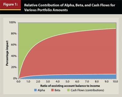
Similar to Table 1, the relative importance of Cash Flows decreases as the account balance increases. Again, this should not surprise the reader. If we assume the hypothetical investor is saving 6.0 percent of his $100,000 compensation this would be an annual savings amount of $6,000. To produce an equivalent portfolio return, the investor would need to earn 1.0 percent on a $600,000 portfolio (account balance-to-income ratio of 6.0) or a 10.0 percent return on a $60,000 portfolio (account balance to income ratio of 0.6). Following this logic, the relative importance of Cash Flows decreases as the account balance grows.
These results have important implications for different types of investors. For example, Table 1 and Figure 1 could provide insight as to the optimal participant messaging strategy of a plan sponsor for its 401(k) plan. Older investors with larger balances likely should be encouraged to use professionally managed options, such as a target-date fund or managed account(s), because 401(k) participants are notoriously bad investors2. In contrast, younger participants should be encouraged to save. Increased adoption of target-date funds or managed accounts would likely only have a minor impact on younger participants if they are not saving, and ideally, messaging should be created that reflects this fact. This research is not suggesting older participants with larger balances should not save. Savings represents a form of account growth that is a “free lunch,” unlike Alpha and Beta, which are uncertain in both the short and long term.
Retirement Analysis
The objectives of accumulation and retirement are different. Accumulation is focused on saving, and retirement is focused on spending. But both are based on the same goal—replacing income when an individual stops working. While the accumulation analysis focused on the impact of Alpha, Beta, and Cash Flows on the change in an investor’s account balance over a year, the retirement analysis uses a goal-based measure to determine each factor’s respective impact; namely, the probability of success.
The probability of success is a very common metric in retirement research. It is usually calculated through stochastic simulation (that is, Monte Carlo analysis3) and represents the number of runs where the retiree achieves his or her goal divided by the total number of runs simulated. The higher the probability of success the better.
For example, assume a hypothetical retiree has a $1 million portfolio and a goal to generate $40,000 of income a year, adjusted annually for inflation, for 30 years. If the goal was accomplished 9,000 times within a 10,000 run simulation, the probability of the retiree achieving this goal would be 90 percent. This means the retiree would have achieved this spending goal for 90 percent of simulations. This does not mean the retiree has a 90 percent probability of achieving the goal, as market conditions are unknown, but rather represents an estimate of the likelihood of achieving a goal given the base assumptions.
The multivariate regressions for this retirement analysis differ slightly from the accumulation analysis because a constrained regression is used to determine the regression coefficients versus a pure multivariate regression. The objective for the constrained regression is the same: to minimize the sum of the squared errors. A constrained regression is performed because the outcome itself is constrained, as the probability of success is bounded between 0 percent and 100 percent. Therefore, for the constrained regression, the sum of the squared errors is minimized subject to the constraint that the resulting probability of success is bounded between 0 percent and 100 percent. The intercept also is set to 100 percent for simplicity purposes.
One hundred scenarios are considered, each based on a 10,000 run Monte Carlo simulation: five Alpha scenarios (from −2 percent to 2 percent in 1-percent increments), five Beta scenarios (equity allocations from 0 percent to 100 percent in 25-percent increments), and four initial withdrawal rate scenarios (from 2 percent to 8 percent in 2-percent increments).
For the withdrawal rate scenarios, the annual withdrawal is determined by multiplying the initial withdrawal rate by the balance. This amount is then increased each subsequent year by inflation so the cash flow is a constant inflation-adjusted amount. Therefore, while the withdrawal rates are expressed as a percentage, the withdrawal percentage really only applies to the first-year withdrawal, because after the first year the withdrawal amount has already been determined. The results from the regressions are included in Table 2 for 20-, 25-, 30-, 35-, and 40-year periods.
Table 2 reflects the hypothetical respective weights that each percent of Alpha, Beta, and Cash Flows has on a retiree’s probability of retirement success for various distribution periods. For example, if the reader believes that a retiree will live 30 years, achieve an Alpha of 1 percent, a Beta return of 7 percent, and the initial withdrawal rate (Cash Flow) is 4 percent, the probability of success would be determined as 100% + (1% ≈ 11.68) + (7% ≈ 8.54) + (4% ≈ −20.57) = 89.2%. These results are relatively similar to the actual probability of success determined via the Monte Carlo simulation, which was 90.4 percent.
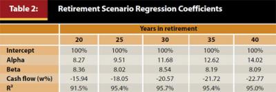
Table 2 provides some interesting takeaways. First, and perhaps most noticeably, while Beta becomes less important over longer periods (slightly), Alpha becomes increasingly important. This can be attributed to the fact there is no variance drain to the Alpha return (versus the Beta return) and therefore the “risk-free” nature of the Alpha return makes it increasingly important for longer periods. Also, while Alpha and Beta are important, a 1 percent change in the initial withdrawal rate (Cash Flow) has a greater impact than a 1 percent increase in return, either Beta or Alpha. Therefore Cash Flows are the most important determinant of retirement success.
Table 2 also has important implications with respect to adviser or financial planning fees, which would be characterized as negative Alpha. If total financial planning and investment management fees are 1.00 percent per year, holding every other variable constant, the probability of success is going to decrease by 11.68 percent for an investor with a 30-year time horizon. Therefore, fees are an important consideration when thinking about the impact of receiving advice on retirement success. We are not suggesting financial planners do not add value, as the initial research by BK on Gamma suggests the contrary; rather, this research suggests that a financial planner should offer services to overcome this cost, such as potentially encouraging a retiree to invest more appropriately, withdrawing less from the portfolio, or by offering additional services that are beyond the scope of this paper.
In addition, Table 2 provides some insight into past research on sustainable withdrawal rates. A researcher who either uses a historical return period with higher returns or uses a higher forecasted return is going to find a higher probability of achieving a goal than other researchers who may have used more conservative return estimates. Depending on the assumed standard deviations, these assumptions could affect either the Alpha regression coefficient with respect to Table 2 or the Beta coefficient. In either case, Table 2 clearly demonstrates that research using higher return assumptions generally should be expected to promote higher withdrawal rates (Cash Flows) and vice versa.
Figure 2 has been included to provide the reader with an idea of how the magnitude of the relative factors can change through time for retirement. Figure 2 uses the same Alpha (+0.5 percent) assumption as Figure 1, although a slightly lower Beta assumption (6 percent versus 7 percent) to reflect the fact retirees tend to invest more conservatively. The initial withdrawal rates (Cash Flows) for each period are based on the formula where the Cash Flow (initial withdrawal percentage) is: 1/time period. For example, if the period is 30 years, the initial withdrawal would be 3.33 percent (1/30=3.33%). This withdrawal approach is similar to the amount that must be withdrawn from accounts such as 401(k) plans that are subject to Required Minimum Distributions (RMDs). The efficiency of the RMD has been noted in past research by Blanchett, Kowara, and Chen (2012) as well as Sun and Webb (2012).
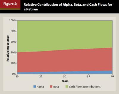
There is little change in the relative contribution or importance of the three factors in Figure 2 when compared to Figure 1. One noticeable aspect of Figure 2, though, is that the relative combined importance of Alpha and Beta (the return portion) is roughly equivalent to the Cash Flow importance by year 40. This can be attributed to the fact that the longer the portfolio duration, the lower the likely initial withdrawal and the greater importance the actual returns will have on determining whether or not the retiree’s goal is actually achieved. This fact reflects the importance of retirees to maintain some percentage of their account balance in investments that have a higher expected return, such as equities (versus bonds).
Delayed Retirement Analysis
The previous analysis considered the impact of Alpha, Beta, and the impact of Cash Flows on the likelihood of an investor achieving a successful retirement. In this section, a fourth variable is introduced: Delayed Retirement.
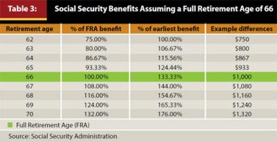
Delaying retirement can have significant positive implications on the likelihood of achieving a successful retirement. This improvement stems from two things: more assets and a decreased retirement liability (or income need). Assets at Delayed Retirement should be higher because an investor’s portfolio has had more time to grow and there should be additional savings. The income needed from the portfolio, or liability, should be lower because the retirement period is going to be shorter and the funding needs from the portfolio also should have decreased because of a higher Social Security retirement benefit. This concept is addressed in a book by Munnell and Sass (2008), whose title Working Longer: The Solution to the Retirement Income Challenge sums up the potential benefits of Delayed Retirement. They noted that delaying retirement just four years, from age 62 to age 66, can increase retirement income by 33 percent.
The optimal age to claim Social Security retirement benefits is a complex analysis and beyond the scope of this paper. However, delaying Social Security retirement benefits can have a significant impact on a retirement success. The “Full Retirement Age” (FRA) is age 66 for those workers born between 1943 and 1954, which is the FRA assumed for this analysis. An individual can claim Social Security retirement benefits as early as age 62 (four years before FRA) or wait until age 70 (four years after FRA). A retiree can technically claim benefits after age 70, although there is no benefit to delaying benefits past age 70 because the benefits will not increase. The benefit from claiming Social Security benefits early is the income starts sooner. The benefit from delaying is the eventual benefit will be higher. The impact on the benefit is included in Table 3. There are additional considerations not included in this analysis, such as spousal survivor benefits, which increase the effective benefit to delaying Social Security benefits, and the impact of earnings on benefit taxation, but both are beyond the scope of the analysis.
The following analysis demonstrates the impact delayed (or early) retirement has on the probability of success. The portfolio value is assumed to be $825,765 four years prior to retirement. The hypothetical worker, making $100,000 per year is assumed to be saving 8.0 percent per year ($8,000). Given a nominal return of 6.5 percent, which corresponds to a real (inflation-adjusted) return of 4.0 percent, the portfolio would be expected to grow to approximately $1 million (in today’s dollars) at age 66, which is FRA for this individual. The target income goal is $65,000 per year during retirement, increased annually by inflation. The retiree is assumed to receive a $25,000 Social Security retirement benefit at age 66 (in today’s dollars), therefore, at FRA the portfolio withdrawal amount would be $40,000 ($65,000 − $25,000 = $40,000, in today’s dollars), which represents an initial withdrawal rate (Cash Flow) of 4 percent. Given this goal and these assumptions, it is possible to determine the impact on the probability of achieving this goal based on different delay periods.
Should the individual choose to retire four years before FRA, at age 62, the Social Security benefit would be 75 percent of the FRA benefit, or $18,750 per year. This means the annual income needed from the portfolio would be $46,205 (versus $40,000 at FRA). Additionally, the portfolio would only be valued at $825,765 (the starting amount), versus approximately $1 million (which is the approximate amount the account would grow to at FRA). This means the portfolio withdrawal rate is 5.6 percent at age 62 versus 4.0 percent at age 66. Figure 3 includes the probabilities of success for various retirement periods based on different years of delay.
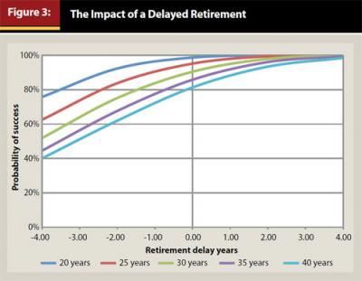
As seen in Figure 3, delaying retirement can significantly improve the probability a hypothetical retiree will achieve his or her retirement goal, which in this example was based on a 4 percent Cash Flow (initial withdrawal rate). Similar to the previous retirement test, a constrained regression analysis is performed to determine the impact of a delayed retirement on the probability of retirement success. The Alpha, Beta, and Cash Flow assumptions were the same as those used in the previous retirement analysis, but five different delay periods were added for a total of 500 scenarios: four years early (−4), two years early (−2), no delay (0), two-year delay (+2), and four-year delay (+4). The same constrained regression process was used, where the sum of the squared errors was minimized subject to the constraint the resulting probability of success could be no less than 0 percent and no more than 100. The results of the constrained regressions are included in Table 4.
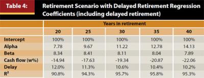
Delaying retirement has a significant, positive effect on the probability of success for a hypothetical retiree. All things considered, delaying retirement one year increases the probability of retirement success by approximately 10.6 percent over a 30-year period. To put this 10.6 percent improvement in retirement success in context, adding 1.0 percent Alpha per year over the 30-year retirement period has the same approximate contribution to success (11.22 percent versus 10.6 percent). If an adviser charges 1.0 percent per year for his or her services (which would be negative Alpha in the context of this paper), by convincing a client to delay retirement by just one year the adviser will have effectively “paid” for his or her services over the next 30 years, ignoring any future Alpha, Beta, or additional financial planning contributions. Additionally, reducing the initial Cash Flow (withdrawal rate) by 0.5 percent would have the same approximate affect.
Conclusions
Past research by Blanchett and Kaplan (2012) introduced the concept of “Gamma,” which is a metric designed to quantify the potential benefits that an investor can realize from making intelligent financial planning decisions. This paper continued this line of research, but focused on quantifying the relative importance of four concepts called the “ABCDs of Retirement Success.” These factors are Alpha, Beta, Cash Flows (contributions for accumulators and distributions for retirees), and the benefits of Delayed Retirement.
This paper explores relative importance of each of these factors for various scenarios. This is done through multivariate regressions and constrained optimizations with the resulting finding that while each of the different factors considered is important, they are not equally important, and they affect outcomes differently, and that for a hypothetical investor nearing retirement, delaying retirement a single year can increase the probability of success by approximately 10.6 percent, or the approximate equivalent to generating 1.0 percent of Alpha during each year of the entire retirement period.
Endnotes
- Results from the simulations described are hypothetical and not actual investment results or guarantees of future results. This should not be considered tax or financial planning advice.
- See Benartzi (2001) for over allocation to employer stock, and Barber and Odean (2000) for individual investor performance.
- Monte Carlo is an analytical method used to simulate random returns of uncertain variables to obtain a range of possible outcomes. Such probabilistic simulation does not analyze specific security holdings, but instead analyzes the identified asset classes. The simulation generated is not a guarantee or projection of future results, but rather, a tool to identify a range of potential outcomes that could be realized. The Monte Carlo simulation is hypothetical and for illustrative purposes only. Results noted may vary with each use and over time.
References
Barber, Brad M., and Terrance Odean. 2000. “Trading is Hazardous to Your Wealth: The Common Stock Investment Performance of Individual Investors.” Journal of Finance 55 (2): 773–806.
Benartzi, Shlomo. 2001. “Excessive Extrapolation and the Allocation of 401(k) Accounts to Company Stock.” Journal of Finance 56 (1): 747–764.
Bennyhoff, Donald, and Francis Kinniry Jr. 2010. “Advisor’s Alpha.” Vanguard research paper (December). https://advisors.vanguard.com/iwe/pdf/ICRAA.pdf?cbdForceDomain=true.
Blanchett, David and Jason Grantz. 2011. “Retirement Success: A Surprising Look into the Factors that Drive Positive Outcomes.” The ASPPA Journal 41 (3): 6–11. www.unifiedtrust.com/new/documents/PositiveOutcomesFactorsv43.pdf.
Blanchett, David, and Paul Kaplan. 2012. “Alpha, Beta, and Now … Gamma.” Morningstar White Paper (December).
Blanchett, David, Maciej Kowara, and Peng Chen. 2012. “Optimal Withdrawal Strategy for Retirement Income Portfolios.” Retirement Management Journal 2, (3): 7–20.
Munnell, Alicia H., and Steven Sass. 2008. Working Longer: The Solution to the Retirement Income Challenge. Washington, D.C.: Brookings Institution Press.
Scott, Jason. 2012. “Household Alpha and Social Security.” Financial Analysts Journal 68 (5): 6–10.
Sun, Wei, and Anthony Webb. 2012. “Can Retirees Base Wealth Withdrawals On the IRS’ Required Minimum Distributions?” Center for Retirement Research Issue in Brief.
Citation
Blanchett, David M. 2013. “The ABCDs of Retirement Success.” Journal of Financial Planning 26 (5): 38–45.