Journal of Financial Planning: May 2011
David M. Blanchett, CFP®, CLU, AIFA®, QPA, CFA, is the director of consulting and investment research for the Retirement Plan Consulting Group at Unified Trust Company in Lexington, Kentucky.
Executive Summary
- The portfolio construction process has historically yielded a two-dimensional output, where the efficiency of a portfolio is determined based on its return and the standard deviation. Risk is usually defined as standard deviation and based on a single holding period: annually. This approach to portfolio construction ignores the fact that investors have varied investing time frames.
- This research will demonstrate that the relative efficiency of a portfolio changes over various holding periods, and that by adding a third dimension to the optimization process—time—you can create portfolios that are more efficient given an investor’s expected holding period.
- An approach is introduced to incorporate time into the efficient frontier, which allows the user to easily adjust the input parameters for mean-variance optimization (MVO) through the use of a simple “time decay” factor.
- This approach has practical implications when building portfolios, such as determining the allocations in a “bucket” portfolio and determining the equity glide path for a target-date portfolio.
“Time changes everything.”
—Thomas Hardy
The portfolio construction process has historically yielded a two-dimensional output, where the efficiency of a portfolio is determined based on its relative return and standard deviation. Risk is based on a single holding period (usually annually) regardless of the expected holding period of the investor (for example, 1 year or 20 years). This approach ignores the fact that the relative efficiency of a portfolio changes over various holding periods, and that by adding a third dimension to the optimization process—time—you can create portfolios that are more efficient given an investor’s expected holding period.
This paper will introduce an approach to incorporate time into the efficient frontier. This approach allows the user to easily adjust the input parameters for mean-variance optimization (MVO) through the use of a simple “time decay” factor, where the annualized standard deviations are reduced at some constant rate. The methodology results in efficient portfolio allocations that vary across time periods. This approach has practical implications when building portfolios, such as determining the allocations in a “bucket” portfolio and determining the equity glide path for a target-date portfolio.
Standard Deviation as a Proxy for Risk
While there are many ways to quantify risk, standard deviation is the most popular. Mathematically, standard deviation is the square root of the average squared variance of a given data set from its mean. The resulting statistic, the standard deviation, gives the user an indication of the dispersion of the data assuming a normal distribution (or “bell curve”). For example, if we assume an average equity return of 10 percent with a standard deviation of 20 percent, we would expect approximately 68 percent of all return values to be within –10 percent and +30 percent (within one standard deviation) and approximately 95 percent of all return values to be within the –30 percent to +50 percent return range (within two standard deviations).
Standard deviation has remained a popular definition of risk for a variety of reasons: it is computationally simple, it is widely known, it allows the user to determine the likelihood of a range of outcomes based entirely on two data points (the average and the standard deviation), and it is scalable across periods. For example, if you multiply the daily (monthly) market standard deviation of 1.05 percent (5.43 percent) by the square root of 250 (12), which is the number of trading days (months) in a year, you get an annualized standard deviation of 16.60 percent (18.81 percent), which is a reasonable approximation for the actual annual standard deviation of 20.50 percent.
There has been some debate as to whether standard deviation is an appropriate measure of risk for investments, particularly equities, because many types of investments have non-normal return distributions (do not fit the “bell curve”). Standard deviation does an especially poor job describing equity returns over shorter periods (such as daily). For example, from January 1, 1925, until December 31, 2009, the arithmetic average daily return of the CRSP value-weighted total market index was .04 percent with a standard deviation of 1.05 percent. Given a daily average return of .04 percent (10.51 percent annually) and a daily standard deviation of 1.05 percent, the probability of a daily return being greater than 7 percent or less than –7 percent is less than one in a billion, assuming daily returns are normal. However, during the 22,204 days of the test period there were 34 days with returns outside this range, which corresponds to .15 percent of the days during the period; the most notable being the return on Black Monday, October 19, 1987, of –17.13 percent. These results would suggest that standard deviation is a poor descriptor of daily returns.
There are numerous ways to determine whether a return distribution is normal, such as a test of the studentized range or a review of the descriptive statistics such as skewness and kurtosis. However, one of the simplest and most revealing tests is to review a histogram of the return distribution of a data series against the normal bell curve to see how well the returns fit a normal return distribution. Figure 1 includes such a study, in which the daily, monthly, and annual return distributions of the CRSP value-weighted total market index (the “market”) from January 1, 1925, until December 31, 2009, as well as the annual real returns for Jeremy Siegel’s data set from 1802 to 2009, are plotted against a normal distribution.
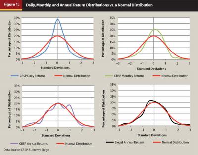
As the reader can see from Figure 1, the daily and monthly return series do a poor job “fitting” the normal distribution. The daily and monthly return distributions are peaked and have fatter tails than the normal distribution, something known as a leptokurtic distribution. However, annual returns, using either the CRSP market data or Siegel’s data set, appear normal, at least to the first approximation. Therefore, while standard deviation does not appear to be a reasonable proxy for daily or monthly returns, it is a reasonable, if imperfect, proxy for annual returns.
Just because the annual equity returns appear approximately normal does not mean that standard deviation is a reasonable definition of risk. In order to be able to use standard deviation as a proxy for risk, it must match what investors perceive as risk when investing. While it is unlikely that standard deviation would have remained popular for so long if it wasn’t a valid risk metric, standard deviation isn’t without its flaws. Standard deviation works poorly with investments that have non-normal return distributions, such as options. Also, while few investors view positive returns, or returns above the minimum acceptable return, as risky, standard deviation “punishes” positive returns as much as negative returns when determining the overall risk of an investment.
Because of the deficiencies of standard deviation, alternative definitions of risk have also become popular, such as shortfall probability and downside risk, which seek to more accurately quantify risk the way investors experience it. However, these definitions are somewhat ambiguous and user-defined, which is why they have been unable to gain the popularity and widespread use of standard deviation. Also, the findings in Figure 1 that annual returns are approximately normal enables standard deviation to be used as an acceptable measure of risk.
Time Diversification
Equities are an attractive investment because they have historically yielded higher average returns than bonds or cash. The higher expected return, though, has been accompanied by higher levels of risk, or a higher standard deviation. The longer an investor holds equities, though (or cash or bonds), the more the compounded average return tends to converge toward the long-term average (this is explored next). This mean reversion has given rise to the notion of “time diversification” whereby the risk of investing in equities is assumed to decrease as the holding period increases. This concept is displayed visually in Figure 2, which includes the historical real (inflation-adjusted) maximum and minimum annual compounded returns for cash, bonds, and stocks from 1802 to 2009 (based on Siegel’s data set) for various holding periods.
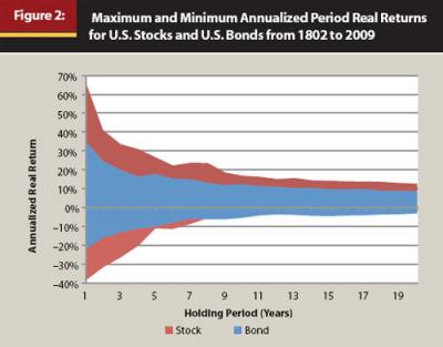
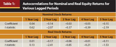
As the reader can see in Figure 2, over longer periods the maximum and minimum annualized real returns for stocks and bonds have converged toward their long-term average. This is because the historical returns of stocks and bonds have been somewhat “stationary,” or have tended to drift around some mean return (in other words, are mean reverting). This suggests that the returns exhibit some degree of negative autocorrelation (or negative serial correlation) whereby the return in future years tends to be negatively related to the return in the past year (for example, if the market was down last year it is likely to be up the next year). This concept is displayed in Table 1.
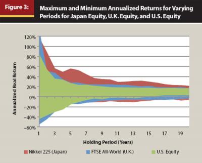
The general convergence of long-term returns for U.S. stocks and bonds in Figure 2 also holds internationally. Figure 3 includes historical performance for Japan (as defined as the annual nominal price return of the Nikkei 225 from 1914 to 2009) and the United Kingdom (as defined as the annual nominal price return of the FTSE All-Share Index from 1800 to 2009).1 As the reader can see from Figure 3, U.S. equities have historically had a tighter return distribution than U.K. equities or Japan equities.
Using the same data set used for Figure 2, numerous lagged autocorrelation tests were conducted on the nominal and real annual equity returns from 1802 to 2009 using the Siegel data set for the various lagged periods. The results are included in Table 1.
The results in Table 1 suggest that returns are somewhat mean reverting after the first year. However, the idea that the risk associated with investing in equities decreases over time is still up for debate and depends largely on how the definition of risk is framed. If “risk” is the likelihood of not achieving a certain annualized return (in other words, replicating the input for a mean-variance optimization) then the results in Figure 2 and Table 1 suggest that equity risk does decrease with time; however, if equity risk is defined in terms of the cumulative total return (in other words, the terminal wealth the investor actually experiences), then the risk of equities actually increases with time. This concept is displayed visually in Figure 4, which includes the maximum and minimum cumulative total period real returns for stocks and bonds from 1802 to 2009 for various holding periods.
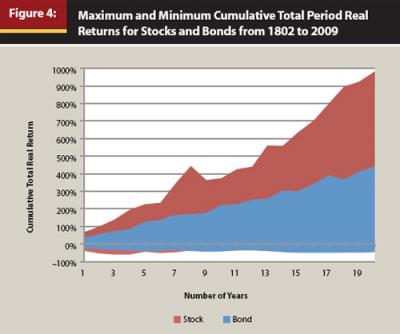
Comparing Figure 2 with Figure 4, the reader will note that in Figure 2, the annualized returns tend to converge over time. In Figure 4 the cumulative returns tend to diverge over time. From a cumulative wealth perspective, the risk of investing increases, not decreases, over longer periods because of the effects of compounding. The standard deviation of the total continuously compounded returns increases in proportion to the square root of the time horizon, which is defined mathematically as: t.5 x σ, where t equals the number of years and σ is the annual standard deviation. For example, a 16-year investment is four times as uncertain as a 1-year investment if we measure “uncertainty” as the standard deviation of continuously compounded total return (16.5 = 4, which would be multiplied by the annual standard deviation, which would be a constant regardless of the time period for the equation).
The “increasing” risk perspective of time diversification may seem counterintuitive to many investors given the widespread acceptance of the concept of time diversification. Bodie (1995), among others, though, has demonstrated this relationship by referencing the nature of option pricing using the Black-Scholes equation. Despite the fact that the probability that stocks will earn less than the risk-free rate decreases with the length of the time horizon, the cost of insuring against this underperformance increases for longer periods. Or simply, longer-dated options tend to cost more than shorter-dated options (if you don’t believe the author, just look at option prices on the same security for the same strike price for varying maturities and you’ll see the longer-dated options cost more). If equity risk decreased through time, the entire options market would be mispriced.
So does time diversification exist? It depends on your definition of risk. The dispersion in returns away from the long-term average decreases for equities over longer periods (time diversification does exist), yet the impact on your cumulative wealth increases for equities over longer periods (time diversification does not exist). If you define risk as achieving the historical annualized return (replicating the return in an optimizer), then you could argue time diversification does exist, whereby historically the longer equities are held the greater the likelihood of achieving the long-term average. However, if you define risk as the cumulative return (terminal wealth) of an investor, then you could argue time diversification does not exist.
The Efficient Frontier
The fundamental goal of portfolio theory is to determine the optimal allocation among different assets. While there are many methods to determine an optimal allocation, mean-variance optimization (MVO), developed by Harry Markowitz (1952), is the clear industry favorite. Two key reasons traditional MVO remains popular are its aesthetic appeal and its relative simplicity. A traditional MVO optimizer creates only one efficient frontier, which allows the user to easily compare the relative efficiency of two or more portfolios. MVO is also relatively simple in that it only takes a basic understanding of financial markets to adjust the input parameters to create and/or determine efficient portfolios.
The goal of MVO is relatively straightforward: to help the user determine “efficient” portfolios. A portfolio is efficient, according to Markowitz’s original research, if “no other portfolio has a higher expected return for a given level of risk or less risk for a given level of expected return.” Three primary inputs are required for MVO: returns, standard deviations, and correlations. These estimates combine to create the “efficient frontier” depicted in Figure 5, which are those combinations of investments with the highest return per unit of risk.
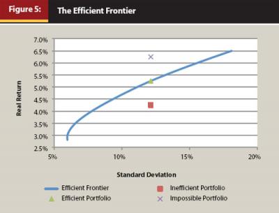
MVO is not without its faults, though. MVO often results in impractical allocations with exaggerated exposures to a relatively small number of asset classes, which cannot reasonably be expected to be implemented for clients. MVO is also highly sensitive to inputs, where slight changes to the inputs can lead to dramatically different outcomes. If the user were able to perfectly predict future returns, this would not be a problem; however, it is likely that there will be a difference in the forecasted values and the actual values, which creates what is known as “estimation error.” A user can do various things to minimize estimation error—simple things such as using constraints (for example, no shorting and maximum allocations) or more advanced things like resampling, a process originally introduced by Jorion (1992) and expanded on greatly by Michaud (1998) that introduces uncertainty into the optimization process through a simulation analysis.
A Multi-Period MVO Model
Mean-variance optimization (MVO) is a single-period model, yet the period can be defined entirely by the user. Despite this flexibility, annual inputs are most commonly used as the period. The user could just as easily select a shorter period (daily values, for example) or a longer period (20 years, perhaps). While shorter periods may be of concern to larger, more institutional-type investors, such as a bank calculating its daily value at risk, returns become increasingly non-normal over shorter periods, which makes standard deviation a less useful definition of risk. Also, a financial planning client with an investment horizon of less than a year should usually be invested very conservatively.
This paper will explore the implications of using periods longer than a year for MVO. For example, if an investor has a 10-year investing horizon, is the efficient portfolio the one that minimizes the risk (variance of return) for a 1-year period or for the entire investment period? While it’s true that investors “experience” risk and performance frequently (as often as daily), the goal of a portfolio should be to achieve a desired outcome with the minimum amount of potential return dispersion; therefore, length of the investment holding period should be considered when constructing the optimal portfolio.
If the efficient allocation did not change for different periods, incorporating time into the efficient frontier would be of no consequence; however, as will be demonstrated in this paper, this is not the case. Over longer periods equities become increasingly efficient, and some of the lowest-risk portfolios can actually have greater return distributions (in other words, more risk) than more diversified portfolios. Before we can build portfolios over varying time periods we must determine the appropriate risk inputs for the MVO.
Determining Time Decay
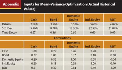
Five asset categories are considered for the analysis portion of the research: cash, bonds, domestic equities, international equities, and real estate.2 All returns are converted into “real” terms (inflation-adjusted) using the definition of inflation from Siegel’s data set. Real returns are used because they represent the return experienced by an investor after allowing for loss in purchasing power through inflation. Using real returns also reduces the autocorrelation associated with annual cash returns (which exhibit significant positive autocorrelation). However, changing the nominal returns into real returns tends to increase the correlations across asset categories because each return series is being divided by the same inflation rate.
Given the scalable nature of standard deviation, we would expect the returns of the five asset categories to experience the same “time decay,” or reduction in risk over time. This time decay figure can be calculated by dividing the annual standard deviation by the square root of the number of years of the holding period (in other words, a time decay factor of .5). For example, if the annual standard deviation were 20 percent, we would expect the standard deviation of returns to be 10 percent for a four-year investment period (20% / (4 ˆ .5) = 10%) and 5 percent for a 16-year investment period (20% / (16 ˆ .5) = 5%). However, as will be demonstrated, the historical time decay exponents have varied from the expected value of .5.
In order to correctly describe the “time decay” associated with the five data series, a calculation was performed using the Solver function in Microsoft Excel to determine the exponent that minimizes the sum of the squared errors for the differences between the approximated standard deviations and the actual standard deviations for the different holding period years. Holding periods from 1 to 20 years are considered in 1-year increments. Standard deviations for each asset category were calculated using rolling, overlapping periods with all available data.
The exponent in the traditional calculation to reduce the standard deviation over varying time periods is .5, which is the same as dividing a number by the square root. While the expected time decay factor of .5 did a reasonable job describing the reduced volatility in bonds and domestic equities over time, it overstated the reduction in risk for bonds and understated the reduction in risk for equities. It was determined that the appropriate “time decay” factor was: .27 for cash, .36 for bonds, .60 for domestic equity, .60 for international equity, and .69 for real estate.
An exponent less than .5 (for example, for cash and fixed income) suggests that the risk of that asset class decreases at a slower rate than expected, while an exponent greater than .5 (for example, for domestic equity, international equity, and real estate) means risk decreased at a faster rate than expected. It is worth noting that while the more precise time decay estimates will be used for the remainder of the paper, adjusting the time decay factor does not materially affect the results of the optimization; reducing the standard deviation of the asset class through time is far more important.
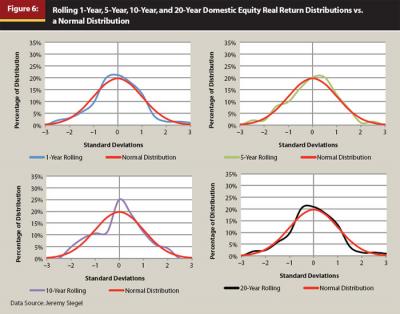
If standard deviation does a poor job describing returns over longer holding periods, this approach would not necessarily be valid. However, similar to Figure 1, Figure 6 includes charts with the rolling 1-year, 5-year, 10-year, and 20-year domestic equity real return distributions versus a normal distribution. Figure 6 demonstrates that while not perfectly normal, annualized returns over various holding periods from 1 to 20 years are approximately normal, and therefore standard deviation can be used to reasonably describe their distributions.
Incorporating Time into the Efficient Frontier
Now that we have an appropriate methodology to determine how the risk for various asset categories changes over varying holding periods from 1 to 20 years, it is possible to build efficient frontiers for each period. Because the length of the period of investment is going to change across holding periods, for simplicity purposes, the historical annualized return (the geometric mean) for the investment period is used as the MVO input for return. While the standard Markowitz algorithm states the user should use the arithmetic mean, the geometric mean is used instead to incorporate the loss of return associated with higher levels of standard deviation. Worth noting, though, is that the Markowitz algorithm with arithmetic mean inputs will always overestimate the true return of any given rebalanced portfolio, while the same algorithm using geometric mean inputs will always underestimate the true return.
Because the international equity data and real estate data cover a different time period than the cash, bond, and domestic equity data, an adjustment was made to “standardize” the annualized real return for the two data sets for the MVO. The annualized real return of domestic equity from 1972 to 2009 was approximately 2 percent less than the full-period annualized return (4.57 percent versus 6.53 percent, respectively); therefore, it is likely the returns for international equity and real estate are lower as well (and would therefore be higher if full-period returns were available). In order to assign an appropriate full-period return to these two asset classes, a CAPM estimate methodology is used in which the beta of the respective returns against domestic equity was calculated (.86 for international equity and .74 for real estate), and this number is multiplied by the total-period return of domestic equity to get the respective returns for each asset class. The author acknowledges this is an imperfect approach, but considered it the most reasonable way to match the test periods.
The annualized standard deviations and correlations for each asset category are based on the full-period data. No adjustment was made to the international equity and real estate standard deviations, even though they cover shorter periods, because the standard deviation for domestic equity was nearly identical during the shorter sub-periods as during the full test period. Unlike the standard deviations, though, which change based on the holding period, a single set of annual correlations was used for the analysis. Similar to the returns, the correlation inputs in an MVO are average period estimates. As has been demonstrated by Coaker (2006), the correlations across investments are constantly changing across time (somewhat similar to returns, especially over shorter periods). Standard deviation is the only “fluid” MVO input that would change for different periods because the return and correlation inputs tend to be long-term average estimates, not measures of dispersions. No constraints are imposed on the optimizations.
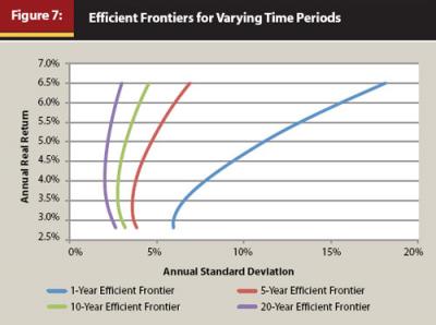
Using the input values in the appendix, efficient frontiers were created for 1-year, 5-year, 10-year, and 20-year periods, and are included in Figure 7. While the actual “efficient” part of the efficient frontier is really only the upward-sloping section of the curve past the inflection point, the entire curve has been included for visualization purposes. Also demonstrated in Figure 7, the relative efficiency of a portfolio can clearly change over varying holding periods. For example, the minimum-risk portfolio for the 1-year period had a return of 2.88 percent, while the minimum-risk portfolio for the 10-year period had a return of 3.67 percent. The allocations for the minimum standard deviations portfolios for each of the 20 test periods are included in Figure 8.
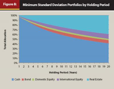
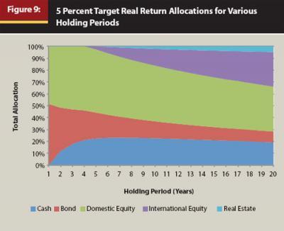
When the definition of risk is changed from one year to more than one year, the allocation with the “least” risk, or expected total variation for the entire holding period, changes considerably. The portfolios in Figure 8, though, have different historical returns. Figure 9 includes similar information to Figure 8, although each of the portfolios in Figure 9 has the minimum amount of risk and a historical real return of 5 percent for a given holding period. Again, the differences in the allocations are striking over time, even more so than the minimum risk portfolios in Figure 8.
The results in Figure 8 and Figure 9 have significant implications for building efficient portfolios. The “minimum-risk” portfolio can change across holding periods. Using the standard one-year model, an optimizer is going to determine that an almost all-cash portfolio is the portfolio with the least amount of risk; this should make intuitive sense to the reader. However, when you incorporate time into the efficient frontier by allowing for different holding periods, you can demonstrate that an all-cash portfolio actually is riskier from a total period return distribution than a more diversified portfolio. This should also make intuitive sense to the reader, because longer-term investors are better served having more diversified portfolios.
Implementation
So what does this research mean from a portfolio implementation perspective? First, it speaks to something that most financial planners have always recognized when building portfolios for their clients: different portfolios make sense over different periods. If you segment client assets into different “buckets” based on different investing time horizons or investing durations, the optimal allocation is likely going to vary by bucket. This research creates a straightforward mathematical framework to determine how each of the buckets should be constructed.
The simplest approach to implementing this research would be to adjust the input parameters in a traditional mean-variance optimizer based on the expected investing period (in other words, you don’t have to go out and purchase new software or do much of anything different than you’re currently doing). The annualized standard deviation assumption would need to be reduced by some “time decay” factor based on the expected time horizon or investment duration. This value can either be specified by the user based on how he or she perceives the risk of that investment will change over time, or the traditional time decay factor of .5 can be used for simplicity purposes. For example, if the user believed the standard deviation for the respective asset class was 10 percent and the portfolio duration was going to be 10 years, using the standard time decay factor of .5, the actual standard deviation input in the optimizer would be 3.16 percent ( 10% / (10 ˆ .5)).
Like other MVO inputs, the time decay factor represents the user’s best guess of the future risk environment for the markets. It is very likely these inputs could vary over different periods. The 5-year time decay factor (or even annualized standard deviation assumption) may not be the same as the 10- or 20-year time factor. This methodology applies to more than just bucket portfolios; it applies to any type of portfolio with a distinct investing horizon, such as target-date investments. If the investing period is defined, it’s important to understand the true “efficient” portfolio given the respective period.
Conclusion
Because people invest for periods longer than a year, it makes sense to consider definitions of risk relative to their investing horizons. The research conducted for this paper suggests that the risk of portfolios changes over time. Therefore, the optimal allocations among cash, fixed income, domestic equity, foreign equity, and real estate are not static over varying holding periods. By incorporating a “time decay” factor in the optimization process, it is possible to add a third dimension to the efficient frontier and create portfolios that are more efficient given an investor’s expected holding period. This concept is relatively easy to implement using existing mean-variance optimizers—all the user needs to do is adjust the standard deviation assumption by the appropriate “time decay” factor.
Endnotes
- Price return indices tend to have lower returns than total return indices because they exclude dividends. Dividends are relatively constant, though, so they are not going to materially affect the dispersion of returns through time. The difference in the price and net returns of the EAFE Japan Index is –1.37 percent per year and the difference in the price and net returns for the EAFE U.K. Index is –3.80 percent.
- Annual cash, bond, equity, and inflation return data were obtained from Jeremy Siegel’s website (author of the bestseller Stocks for the Long Run) from 1802 to 2009. The return of the Net USD return of the EAFE Standard Core Index from 1972 to 2009 was used as a proxy for international equity. The return of the FTSE NAREIT U.S. Real Estate Index Series from 1970 to 2009 was obtained from www.nareit.com and used as a proxy for real estate returns.
References
Bodie, Zvi. 1995. “On the Risk of Stocks in the Long Run.” Financial Analysts Journal 51, 3 (May/June): 18–22.
Coaker, William J. 2006. “The Volatility of Correlation: Important Implications for the Asset Allocation Decision.” Journal of Financial Planning 19 (February): 58–69.
Jorion, P. 1992. “Portfolio Optimization in Practice.” Financial Analysts Journal 48, 1 (January/February): 68–74.
Markowitz, Harry M. 1952. “Portfolio Selection.” Journal of Finance 7, 1: 77–91.
Michaud, Richard. 1998. Efficient Asset Management. New York: Oxford University Press.