Journal of Financial Planning: March 2017
David Blanchett, Ph.D., CFP®, CFA, is head of retirement research at Morningstar Investment Management LLC. He is a two-time recipient of the Journal’s Montgomery-Warschauer Award, as well as a winner of the Journal’s Financial Frontiers Award in 2007.
Michael S. Finke, Ph.D., CFP®, is dean and chief academic officer at The American College. He is a two-time recipient of the Journal’s Montgomery-Warschauer Award.
Wade D. Pfau, Ph.D., CFA, is a professor of retirement income at The American College and a principal at McLean Asset Management. He is a two-time recipient of the Journal’s Montgomery-Warschauer Award and host of the Retirement Researcher website RetirementResearcher.com.
Executive Summary
- Recent asset pricing studies have suggested that demand for stocks since 1980 has driven expected returns below their historical average. The current yield of risk-free assets in the U.S. is also well below historical bond yields. This decrease in bond yields coupled with increases in longevity has doubled the cost of funding a real dollar of income in retirement since 1980 for a 65-year-old retiree.
- Many common financial planning practices are sensitive to asset returns, and advisers need to understand the challenges clients will face if high asset prices persist.
- Results from a life cycle planning model showed that savings rates would need to rise sharply for households hoping to maintain the same standard of living in retirement if real asset returns are low.
- An important finding from this study is that a low-return environment would have a negative impact on client spending throughout their life cycle.
- Advisers may need to modify expected returns in planning software to provide clients with more realistic projections on meeting long-term spending goals. This study provides the numbers needed to re-adjust the retirement expectations.
Many financial planning assumptions are based on historical returns; however, these historical returns may not be relevant in the future. Prices of bonds and stocks are much higher than in the recent past, suggesting a greater likelihood that portfolio returns will fall below the assumptions commonly used by planners. This study explored how lower expected returns affect optimal saving and spending during working years, retirement replacement rates, retirement lifestyles, and the cost of bequests.
Advisers face a number of unknowns when selecting the best strategy to help a client meet a financial goal. Future real returns on financial assets are an important unknown that may be seen as following a continuum from reasonably certain (Treasury Inflation-Protected Securities) to unknown (stocks). Advisers need to estimate future returns on riskier securities, and typically draw from past risky asset returns to project the future.
Blanchett, Finke, and Pfau (2013) estimated that the 10-year return on a bond portfolio can be predicted with 92 percent accuracy based on beginning-of-period interest rates. Although interest rates may rise in the future, the value of a bond portfolio itself will fall and reduce the overall return. Stock returns over a 10-year horizon, however, can be predicted with only 27 percent accuracy by using beginning-of-period valuations (10-year Shiller price/earnings ratio). Given the difficulty in predicting future returns, some advisers may assume historical returns.
Academic studies have painted a less rosy picture of the expected reward investors will receive from risky assets in the 21st century. Greenwood and Scharfstein (2013) pointed out that the total market capitalization of U.S. stocks grew from 50 percent of gross domestic product in 1980 to 141 percent in 2007. By October 2016, the ratio was 120 percent. The near tripling of stock prices occurred with only a modest real increase in corporate profitability. In 2007, investors paid 266 percent more for each dollar of corporate earnings than they paid in 1980.
In other words, stocks in 2016 are nearly three times as expensive as they were in 1980 for each dollar of profit. These profits can either be paid to investors through dividends (the dividend yield is less than half its historical average of 4.4 percent, according to calculations using data from Robert Shiller’s website, www.econ.yale.edu/~shiller/data.htm) or reinvested to provide growth. It is also worth noting that the investment management industry is three times larger in 2016 than it would have been if equity valuations had not increased (Greenwood and Scharfstein 2013).
Expected stock returns, according to the capital asset pricing model, are a function of the risk-free rate plus the risk premium (Sharpe 1964). The risk premium is equal to beta multiplied by the excess returns investors require for selecting a security whose future payout is uncertain. Because the risk-free rate on three-month Treasury bills is 3.28 percentage points below the historical average (0.21 percent in 2015 versus 3.49 percent between 1928 and 2015), nominal returns on equities in the future are expected to be 3.28 percentage points lower than the arithmetic historical average of 11.41 percent (assuming the risk premium does not change). Future equity returns may then be projected at 8.13 percent if the equity premium is as high as the historical average. In a comprehensive review of the U.S. equity premium over the 20th century, Fama and French (2002) estimated the expected equity risk premium as a function of the current stock price and both dividend and earnings growth. The only returns an investor can hope to receive from equity ownership are either future dividend payments or growth in future earnings; therefore, it is sensible to see the equity premium as a function of stock price and a firm’s ability to pay money back to investors.
Fama and French (2002) also noted that historical U.S. equity returns can be split into two periods: 1875–1950 and 1951–2000. Between 1951 and 2000, growth in stock prices was 5.89 times greater than the growth in dividends. In earlier periods, stock prices tended to rise in accordance with growth in dividends (or earnings). Recently, stock prices have risen more rapidly than firm earnings. The authors referred to this increase in stock prices as “excess capital gain,” most of which occurred between 1980 and 2000.
Many advisers and clients became accustomed to returns that resulted from this excess capital gain during the 1980s and 1990s. But the rise in stock prices without a rise in stock earnings may have created an expectation of future returns that is inconsistent with the actual returns that stocks can provide at their 2016 valuations. Stocks either need to fall significantly in value (by more than half) in order to maintain the historical equity premium, or investors will need to get used to a lower return on equity investments.
Fama and French (2002) concluded that “the high 1951–2000 return seems to be the result of low expected future returns” (page 658). Low asset returns would increase pressure on advisers who receive compensation through asset fees, as it may appear to clients as though they’re getting less for their money. As recently as 1990, average yield data from the Federal Reserve showed that a client working with an adviser charging a 1 percent fee on AUM would have paid 12.2 cents for each dollar of income on 10-year Treasury bonds. At a 2.36 percent yield, a client pays an adviser 42.4 cents for each dollar of bond income. A client paid 8.85 cents in adviser fees for each dollar of corporate earnings from stock ownership in 1980, and 27 cents for each dollar of earnings in late 2016.
Additionally, advisers must estimate the length of retirement. Although there is little agreement regarding the optimal retirement duration (i.e., 25 years or 40 years), there have been considerable improvements in mortality rates in the last few decades, especially for wealthier Americans. This suggests the length of retirement has increased and is likely to continue increasing if recent trends persist. The combined impact of lower asset returns with long retirements suggests that retirement in 2016 was the most expensive it had been since calculations began in 1980 and would require increased savings, reduced consumption in retirement, a delayed retirement, or some combination of these to achieve a successful retirement.
Implications of High Valuations
This research discussion begins by illustrating why high asset prices and low expected returns will affect the relative cost of funding financial goals. Figure 1 shows the average cost of purchasing $1,000 of bond income from a 10-year Treasury bond by 20-year periods beginning in 1955, as well as the cost of purchasing $1,000 in stock earnings and $1,000 in dividends.
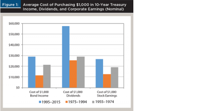
It is substantially more expensive to buy investment income in the modern era than it was in the past. What is most unusual about asset prices in the 21st century is the simultaneous high valuations on risky assets and low yields on safe assets. Safe asset prices were near the low yields of 2016 in a number of historical periods, but these were generally associated with a flight to safety from risky assets (and low price/earnings ratios on these risky assets). The high prices of both stocks and bonds in 2016 are a historical anomaly that is consistent with increased demand for all financial instruments.
The average amount an investor paid for $1,000 of corporate earnings since 1881 was $16,671. Today, an investor must pay $27,812. Since 1927, investors needed an average of $19,802 to buy $1,000 of income from a 10-year Treasury bond. In 2016, an investor needed $42,373 to buy $1,000 of bond income at a 2.36 percent yield. If Treasuries reverted to their historical average of 3.5 percent, the value of a bond portfolio with a 10-year duration would fall by 11.4 percent. The impact of a rise in either interest or dividend income will not prevent investors from facing the consequences of a low-return environment.
Life Cycle Implications
Economists assume that a reasonable goal for most households is to save and spend in a manner that roughly smooths spending over a lifetime. This is the primary motivation for retirement saving. Forward-thinking workers will see that their lifestyles cannot be maintained by Social Security alone, so they will set money aside during working years in order to avoid a drop in spending at retirement.
Saving and spending depends on how much the household earns in the future, how long they can expect to live in retirement, and the expected return on investments. Higher investment returns will allow a household to save less and achieve the same amount in retirement. For example, assume a household earns $50,000 at age 25, expects a 3 percent annual real growth rate in income, and wants $1 million in purchasing power after age 65. If they expect a 5 percent real return on investments, they will save 10 percent of their income each year. If they expect 2 percent, they will need to save 18 percent of their income each year in order to reach their $1 million goal.
When considering the implications of a low-return environment, it is important to remember that the expected portfolio returns are net of inflation and any investment expenses. Given negative bond returns net of asset management fees (average 1 percent) and inflation (0.73 percent in 2015), and expected real equity returns of perhaps 2 percent to 4 percent net of asset fees, it is important to understand the planning consequences of a future 0 percent to 2 percent real portfolio return.
A persistent low-return environment will also impact the amount of income a household can expect to receive from savings at retirement. For example, a $1 million bond ladder will provide $61,954 of income each year until age 95 at 5 percent, but only $38,364 at 1 percent.
A persistently low-return environment both increases the percentage of income a client needs to save in order to meet a retirement goal and reduces the income a client could expect to receive once that goal is reached. This allows a better understanding of some of the potentially counterintuitive results found when the impact of a low-return environment on optimal life cycle saving was estimated.
The life cycle model involved estimating future expected income during working years, spreading the possible resources over a lifetime, incorporating the possible real growth in savings, and solving for the optimal smooth spending amount over time (Modigliani 1966). Because real income grows for most households later in their working years, the savings rate will rise as they get older, but their spending will remain constant. The model used in Table 1 (which includes the results of the analysis) is a simple life cycle model whose moving parts are rate of return, income growth, and desired bequest. This model assumed a discount rate equal to the investment return to keep lifetime spending at a constant real level. More complex calculations appear in Tables 2 and 3.
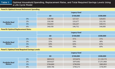

Panel A shows the optimal annual life cycle spending amount at various real expected rates of return for a simplified case study. This analysis considered a 35-year-old individual who earns $50,000 and will experience real wage growth of 1 percent per year for a 30-year career, which is then followed by a 30-year retirement. The most obvious impact of lower expected returns is the reduction in average lifestyle. With no legacy goal, optimal annual spending at a real return of 0 percent is $28,988, compared to $46,938 with a 6 percent expected rate of return. Because legacy goals were also more expensive to fund in a low-return environment, the spread between optimal annual spending amounts widened further for those wishing to pass on $500,000 at death ($20,655 versus $46,008). These were the maximum spending amounts that could be enjoyed consistently over the life cycle for someone working through a 30-year career, saving for a 30-year retirement, and preserving a desired legacy amount. Funding the legacy goal costs little in terms of lifestyle when rates of return are high, but presents a significant lifestyle trade-off when rates of return are low.
Panel B reveals that the optimal retirement income replacement rate declines if the household’s goal is to smooth annual spending. This is consistent with the drop in overall lifetime spending brought about by a low-return environment. Advisers need to consider the need to adjust replacement rates downward if they anticipate a low-return environment during the retirement planning process—particularly if the retirement portfolio has a lower risky asset allocation (and lower expected return) than the pre-retirement portfolio. While optimal replacement rates at a 6 percent real portfolio return are near the 70 percent replacement rate common in planning practice, a 2 percent real portfolio return will result in optimal replacement rates of just over 50 percent with no legacy goal. At a 0 percent real portfolio return, the optimal replacement rate is, a perhaps surprisingly low, 31 percent with a $500,000 legacy goal.
Households will need to accumulate more wealth to maintain even their lower level of lifetime spending in retirement, assuming the low-return environment persists. However, they will need to have a higher savings goal amount in order to sustain that lower level of retirement spending—particularly if they hope to leave a legacy.
Panel C shows that to reach the same level of retirement spending provided by about $750,000 in savings (with a $500,000 legacy) at a 6 percent real return, a household would need to save about $1 million in a 2 percent real return world. Taken together, the three panels of Table 1 show how a low-return environment creates drag on both the accumulation and decumulation portions of retirement planning.
Changes in Longevity
Today’s workers who expect to retire at the same age as retirees in previous generations will face an even greater cost of funding retirement because of increases in longevity after the age of 65 (Society of Actuaries 2016). Retirement is significantly more expensive in a low-return environment, and funding additional years of longevity after retirement further contributes to the savings needed to fund a given level of retirement income.
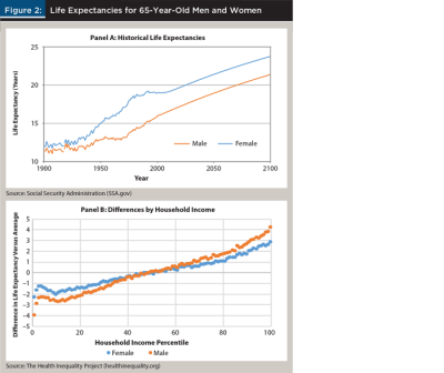
Life expectancies for older Americans have increased considerably over the last 100 years and are projected to continue increasing. Panel A of Figure 2 shows historical and projected life expectancies for 65-year-old men and women in the U.S. The Society of Actuaries 2012 Individual Annuity Mortality Table assumed an annual reduction in the mortality rate of approximately 1 percent per year. Panel B of Figure 2 illustrates how life expectancies vary by household income level, reflecting a relatively recent trend in which higher-income (and wealth) households are living significantly longer than lower-income (wealth) households.
In order to illustrate how both changes in longevity and changes in real bond returns have increased the cost of a safe stream of income at retirement, it is possible to estimate the price of buying $1 in income via an inflation-adjusted annuity through mortality-weighted net present value of cash flows needed to fund average lifetime income.
Figure 3 uses historical mortality tables from the Social Security Administration1, historical Treasury yields from the Federal Reserve2, and historical implied inflation estimates from Cleveland Federal Reserve3 to calculate the cost of funding each year since 1982. True annuity payouts offered by annuity companies differ slightly, although this approach approximates the historical payouts for nominal annuities based on data from ImmediateAnnuities.com.
Figure 3 is a reminder that advisers need to plan for a more expensive retirement. The price of a dollar of safe income for a client retiring in 2016 is nearly 50 percent higher than it was for a client retiring in the year 2000 because of increases in longevity and declines in real bond interest rates.
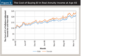
Although the costs of buying a dollar of real income for a lifetime have been increasing, it is important to point out that in contrast to conventional wisdom, annuitization becomes a relatively more attractive option when interest rates are low. This is because the increase in the cost of building a bond ladder is greater than the increase in the cost of buying an income annuity in a low-rate environment. With a bond ladder, retirees spend principal and interest. With an income annuity, retirees spend principal, interest, and mortality credits, which are the subsidies from the short-lived to the long-lived. With interest low in both situations, the mortality credits become more important. Meanwhile, the low discount rate for the bond ladder makes it increasingly expensive, relatively speaking, to fund spending planned for the distant future.
Saving Simulation Model
For advisers interested in understanding how a low-return environment and increases in longevity will affect optimal savings rates for clients, a model was created to estimate the required savings rate needed to maintain the same level of take-home pay during retirement as the final year before retirement. This resulted in different replacement rates by income, because higher savings reduced the take-home pay (and therefore the eventual retirement need).
The retirement income goal was based on the assumption that the individual wants to maintain the level of after-tax (take-home) pay during retirement equal to the after-tax income during the final year before retirement. Retirement was assumed to commence at age 65. The model is similar to Blanchett and Idzorek (2015). All savings were assumed to be pre-tax (e.g., in a traditional 401(k) or IRA). This is a simplifying assumption, because all employer contributions are going to be pre-tax and most individuals save for retirement in sheltered accounts.
Although some financial planning tools may use simple rules of thumb when estimating the income replacement level, such as 70 percent or 80 percent of final gross pay, in reality the number is going to vary significantly by household. The replacement level is generally less than 100 percent, because a number of expenses that individuals incur when working disappear during retirement, such as Medicare taxes, Social Security taxes, and retirement saving, although the impact of these will vary by household. For example, an individual saving 25 percent of her pay before retirement will have a lower take-home pay, and therefore a lower retirement income goal, than an individual saving 5 percent.
Blanchett (2014) found that retirees tended to decrease spending during retirement (after inflation). Annual retiree real income need was assumed to change throughout retirement. Retirees who spend more see a sharper decrease in real spending as they age. This occurs because higher-income retirees have a higher portion of expenditures in discretionary goods and spend less (relatively speaking) at older ages. Incorporating spending curves partially offsets the differentials in the expected length of retirement for different income levels. For example, a lower-income household was forecasted to have a shorter retirement (versus a higher-income household), but their retirement spending as they age would be higher as a percentage of first-year spending than higher-income households.
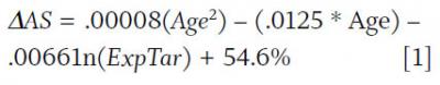
Spending needs in retirement were assumed to follow the equation estimated in Blanchett (2014), which is included as Equation 1 below, where ΔAS represents changes in real retiree annual spending; Age represents age; and ExpTar represents after-tax total expenditures.
Earnings were assumed to change throughout a worker’s lifetime, consistent with distribution differences observed in the data. Earnings curves are especially important for younger workers who are likely to experience significant increases in earnings over their working lifetimes. Because earnings rise, savings were assumed to increase throughout the individual’s working lifetime.
For example, a 25-year-old individual in the 85th percentile would earn approximately $50,000; however, these wages would approximately double by age 50. Without accounting for salary increases, required savings rates for younger workers would be much higher than necessary.
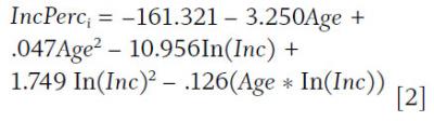
For the analysis, an earnings curve was developed based on data from the University of Minnesota’s IPUMS-CPS (Integrated Public Use Microdata Series for the Current Population Survey) to better replicate how an individual’s earnings are likely to change over a lifetime. The underlying data is from the March 2015 Current Population Survey. To be included in the analysis, the individual had to be coded as employed and working at least 20 hours per week with a minimum annualized income of $5,000. Calculations were made using Excel with Visual Basic. The earnings curves are in 2016 dollars and represent how wages are expected to change over the individual’s working lifetime. The individual’s percentile wages were first determined using Equation 2 (the R2 for Equation 2 was 96.03 percent [adjusted R2 was 95.99 percent], and all coefficients were significant at the 5 percent level):
Wages were then assumed to grow based on the earnings “path” for that percentile using Equation 3 (the R2 for Equation 3 was 93.16 percent [adjusted R2 was 93.09 percent], and all coefficients were significant at the 5 percent level):
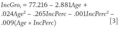
The change was constrained so that it was never greater than 5 percent in absolute terms.
The length of retirement varied depending on the year in which a household expected to retire based on projected increases in expected mortality. Mortality rates used to estimate life expectancy were also adjusted based on the household income percentile. The length of retirement was set so that there was only a 20 percent probability of either member of the household outliving their savings. Mortality rates for single households were based on gender-neutral mortality while mortality rates for a married household were assumed to be one male and one female of the same age.
Social Security retirement benefits were based on the highest 35 years of inflation-adjusted earnings using 2016 bend points values. Taxes were based on the 2016 tax rates for a married couple filing jointly.
The returns for the analysis used an autoregressive model similar to the one introduced by Blanchett, Finke, and Pfau (2013). The return models were calibrated so that one return series approximated the historical averages and included three additional scenarios of low, medium, and high expected returns. The high scenario had returns that were similar to the long-term averages, but incorporated low bond yields. A 50-basis-point portfolio fee was also included, so advisers charging a higher portfolio fee should adjust savings rates slightly upward.
The asset allocation assumed in the model was based on the Morningstar Moderate Lifetime Index glide path. Savings levels were determined by solving for an 80 percent probability of success. Scenarios for historical, moderate, and low asset returns were included. The low and moderate simulations assumed that, for example, bond yields began at a 2 percent real rate of return and either remained low or, in the moderate scenario, rose slowly over time. In the low-bond-return simulation, for example, the mean real return was set at 2 percent, rose to 3.5 percent at the 75th percentile, 5.25 percent at the 95th percentile, and fell to 1 percent at the 5th percentile. In the moderate-return example, the real return rose to 4 percent on average. It should be noted that real bond rates on long-duration corporate securities may fall below the low-return scenario, so these estimates should not be viewed as unrealistically pessimistic.
A common assumption in accumulation forecasts is that deferral rates remain constant as the individual ages (i.e., if the individual is 30 years old and deferring 6 percent, he or she will continue to defer 6 percent of salary until retirement). Total dollar saving may increase if wages are assumed to increase, but investors do not save a constant percentage of compensation.
Using data from 136,250 participants provided by a 401(k) record-keeper as of December 31, 2015, the deferral rate change (DefΔ) throughout the accumulation period was estimated through a multivariate model that included the participant’s age (Age) using Equation 4:
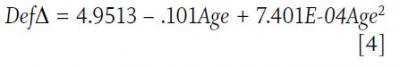
The formula implies that savings rates increase by approximately 25 percent over 10 years. For example, a 35-year-old individual saving 10 percent would be assumed to be saving 12.27 percent at age 45, and 15 percent by age 55.
Finally, improvements in life expectancies are important when estimating the retirement period, because retirement is likely to last longer for an individual who is currently 25 years old and retiring in 40 years, versus an individual who is retiring now at age 65. The base mortality table used for this analysis was the Social Security Administration 2013 Period Life Table. The mortality rates were assumed to decline based on the G2 projection scale in the Society of Actuaries 2012 Individual Annuity Mortality Table.
In addition to general improvements in longevity, higher-income Americans, in particular, are living longer. Waldron (2007) noted that men born in 1941 in the top half of the earnings distribution live 5.8 years longer than men in the bottom half of the distribution (up significantly from the difference of 1.2 years for men born in 1912). Bosworth and Burke (2014) noted a difference in life expectancies of approximately 10 years for men and approximately six years for women between the top and bottom income deciles. This change in longevity for higher-income workers will increase the amount they will need to save to smooth spending in retirement period was 25 percent. Mortality rates for joint couples were assumed to be independent.
Analysis
Table 2 includes target total pre-tax retirement savings rates for households at different starting ages, with retirement assumed to begin at age 65. Each panel assumes that the worker begins saving for retirement at a specific age (25, 30, 35, and 40). Each analysis incorporated expected Social Security, a decreasing spending path in retirement, the impact of taxes, and longevity based on the expected distribution of average U.S. mortality for men and women.
Optimal savings rates using historical data for households that begin saving at age 25 are between 4.3 percent for low earners ($25,000), and up to 9 percent for high earners ($250,000). Assuming more realistic returns (low returns) increased the optimal savings rate by 63 percent to 7.0 percent, and for high earners by 82 percent to 16.4 percent. For most clients of financial advisers, optimal saving simulations in a low-return environment would lead to a recommendation that clients maximize their employer-sponsored retirement contributions even if they begin saving at a young age. This may not be the case if the adviser relies on historical returns to estimate optimal savings.
The results are even more dramatic if households wait to age 35 or 40 to begin saving for retirement. At age 35, optimal savings rates rise to 24.1 percent in a low-return simulation compared to 14.3 percent using historical returns for a single worker. If the household waits until age 40, the optimal savings rate rises to 27.5 percent. Even in a moderate return scenario, optimal savings rates are 24.8 percent for a single household and 22.8 percent for a couple.
The combination of low asset returns and expected increases in longevity mean that households will need to save significantly more in order to maintain spending in retirement. Many clients may be unwilling to accept the lifestyle sacrifices required to save a quarter of earnings. A reasonable alternative is to delay retirement. Postponing retirement increases the number of years of savings (and asset growth), reduces remaining longevity, and increases Social Security income.
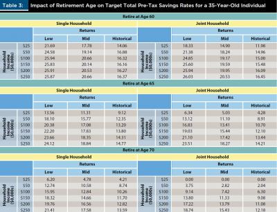
Table 3 shows how optimal savings can be reduced (or lifestyle at present can be improved) by delaying retirement for a household that begins saving at age 35. A couple earning $250,000 would need to each save 26 percent of their income in order to retire at age 60. Delaying retirement to age 70 would reduce the optimal savings rate to a more palatable 18.7 percent. The benefits of deferring retirement are even greater in a low-return environment than they would be if historical returns are used to estimate optimal savings rates. A couple using historical rates would need to save only 16.4 percent of income to retire at age 60 and 12.2 percent if they retired at age 70. An adviser who uses more realistic low-return assumptions to estimate optimal savings rates may be able to provide clients with a more compelling rationale for delaying retirement as an option to improve lifestyle during working years.
Conclusions
Convincing evidence has shown that historically high stock and bond prices will lead to lower future investment returns. The low yield on safe assets, coupled with increases in longevity, has doubled the cost of buying guaranteed income in retirement since 1980. Investors hoping to soften the blow of low safe asset returns by accepting greater portfolio risk are not likely to achieve historical returns on equity investments.
Investors facing inflated asset prices, and the lower expected future returns they imply, must accept the reality that they will need to save more to maintain their lifestyle in retirement. This research showed that a low-return environment plagues both the accumulation and decumulation phases of retirement planning, and the only cure is saving more.
In accumulation, lower returns grow assets more slowly, while in decumulation, lower returns produce less income and assets are used up more quickly than historical rates would suggest. Lower returns in retirement lead to a greater required savings level. More savings and lower returns lead to much higher savings rates.
The steady increase in life expectancy also has led to a need for a larger savings pot at retirement, especially for wealthier workers. Again, this requires more saving today to fund the same income after retirement. Few individuals want to save more because that means spending less today.
A simple and effective response to the need to save more is to delay retirement. Even in a low-return environment, a couple who begins saving 18.7 percent of income at age 35 can maintain their lifestyle in retirement if they delay retirement to age 70.
Advisers using historical asset return data or outdated mortality assumptions may be providing clients with an unrealistically optimistic estimate of either the age at which they can comfortably retire or the amount of savings needed to maintain their current lifestyle. For example, assuming a 30-year retirement period ignores the 43 percent of typical annuity-buying couples in 2014 who were expected to have at least one member live beyond age 95 (Society of Actuaries 2016). When setting a retirement period, 35 or 40 years may be more appropriate for a healthy couple who retires at age 65. Rather than set returns at historical averages, bond returns should be set at today’s yield curve, and equity returns should be adjusted for the lower risk-free rate and reduced equity premium.
The risk of presenting unrealistic scenarios is that clients may believe that they can achieve long-term financial goals without the sacrifices required by the low-return environment. Using historical returns may also mask the potential benefits of strategies that provide greater value in a low-return environment, such as the ability to earn mortality credits through later-life annuitization.
Endnotes
1. See ssa.gov/oact/NOTES/as120/LifeTables_Body.html.
2. See federalreserve.gov/datadownload/Choose.aspx?rel=H15.
3. See clevelandfed.org/en/our-research/indicators-and-data/inflation-expectations.aspx.
References
Blanchett, David. 2014. “Exploring the Retirement Consumption Puzzle.” Journal of Financial Planning 27 (5): 34–42.
Blanchett, David M., Michael Finke, and Wade D. Pfau. 2013. “Low Bond Yields and Safe Portfolio Withdrawal Rates.” Journal of Wealth Management 16 (2): 55–62.
Blanchett, David and Thomas Idzorek. 2015. “The Retirement Plan Effectiveness Score: A Target Balance-Based Measurement and Monitoring System.” Morningstar white paper, available from the authors upon request.
Bosworth, Barry P. and Kathleen Burke. 2014. “Differential Mortality and Retirement Benefits in the Health and Retirement Study.” Brookings white paper, available at brookings.edu/research/differential-mortality-and-retirement-benefits-in-the-health-and-retirement-study.
Fama, Eugene F. and Kenneth R. French. 2002. “The Equity Premium.” The Journal of Finance 57 (2): 637–659.
Greenwood, Robin, and David Scharfstein. 2013. “The Growth of Finance.” Journal of Economic Perspectives 27 (2): 3–28.
Modigliani, Franco. 1966. “The Life Cycle Hypothesis of Saving, the Demand for Wealth and the Supply of Capital.” Social Research 33 (2): 160–217.
Sharpe, William F. 1964. “Capital Asset Prices: A Theory of Market Equilibrium under Conditions of Risk.” The Journal of Finance 19 (3): 425–442.
Society of Actuaries. 2016. “2015 Risks and Process of Retirement Survey.” Available at soa.org/Files/Research/Projects/research-2015-full-risk-report-final.pdf.
Waldron, Hilary 2007. “Trends in Mortality Differentials and Life Expectancy for Male Social Security-Covered Workers, by Socioeconomic Status.” Social Security Bulletin 67 (3): 1–28.
Citation
Blanchett, David, Michael Finke, and Wade D. Pfau. 2017. “Planning for a More Expensive Retirement.” Journal of Financial Planning 30 (3): 42–51.