Journal of Financial Planning; March 2012
Executive Summary
- The authors develop an age-based, three-dimensional distribution model that illustrates a retiree’s yearly transition through retirement, including superannuated years (very old age), to demonstrate the impact of longevity risk
- The model builds on “Probability-of-Failure-Based Decision Rules to Manage Sequence Risk in Retirement” by Frank, Mitchell, and Blanchett (2011) to simultaneously:
» Establish an age-based distribution model
» Incorporate current-age life expectancy
» Address survivorship into superannuated ages
» Address market sequence risk
» Develop a method to rationally incorporate retiree goals of either consumption or inheritance, and switch between the two as desired - Past research has primarily focused on fixed, non-age-specific distribution periods. The model developed in this paper demonstrates:
» How longevity probability can be developed into dynamic, yearly adjustable distribution periods
» These dynamic distribution periods can then be combined with stochastic (Monte Carlo) real returns - The distribution period (DP) can be dynamically managed, as the retiree ages, by varying the percentiles of longevity
- The withdrawal rate is very sensitive to DP, and the DP is very sensitive to life expectancy; thus more attention should be paid to longevity risk than has been in past research
- The probability of failure (POF) remains a useful metric to evaluate exposure of a retiree’s portfolio to market sequence risk, and a POF-based decision rule applies to both the asset allocation effect and the age effect on withdrawal rates
Larry R. Frank Sr., CFP®, is a registered investment adviser with an M.B.A. and B.S. cum laude in physics, living in Rocklin, California. (LarryFrankSr@BetterFinancialEducation.com)
John B. Mitchell, D.B.A., is professor of finance at Central Michigan University. (mitch1jb@cmich.edu)
David M. Blanchett, CFP®, CLU, AIFA®, QPA, CFA, is a research consultant for Morningstar Investment Management in Chicago, Illinois. Blanchett has published more than 30 papers in various industry journals and has an M.B.A. from the University of Chicago, Booth School of Business. (davidmblanchett@gmail.com)
Withdrawal rates are sensitive to two fundamental components: the distribution period (DP) and the market returns’ effect on portfolio values (through the basic formula in which withdrawal rate equals the annual dollars distributed divided by the portfolio value). How do retirement planners separate these two components when helping retirees make decisions about the sustainability of their distributions? Frank, Mitchell, and Blanchett (hereinafter FMB) (2011) described how to measure the market returns component. This paper builds on that work by addressing the distribution period component.
Rather than use generic fixed distribution periods not necessarily associated with a specific retirement age, the authors have developed an age-based model that uses period life table statistics so that life expectancies define the length of the current distribution period (DP) based on the current age of the retiree. The current DP changes dynamically each year as the retiree ages and/or by adjusting the longevity percentile (how long the retiree is expected to live). Additionally, the authors introduce a market sequence risk decision rule in which portfolio withdrawal amounts are adjusted based on market returns.
Brief Overview
This paper develops an age-based, three-dimensional distribution model for retirement. The model plots the results of many simulations relative to each other—each simulation represents a transient state a retiree may dynamically pass through as time and portfolio values change. The concept of transitory states suggests a dynamic process of change the retiree’s decumulation goes through over time and market changes. A range of transient states is okay for a retiree, but beyond that range, spending retrenchment (with bad market returns, commonly referred to as sequence risk) is recommended to increase the probability the portfolio does not fail during that DP. The transient state concept was initially developed and explained by FMB (2011).
The lack of a specific distribution period based on the retiree’s current age is problematic because, as the authors will show, withdrawal rates are sensitive to distribution periods. What is an age-appropriate DP? The model here removes much of this DP uncertainty. The authors also evaluate the transition between “early” retiree ages (with corresponding expected longevities) to “older” retiree ages (superannuated); specifically, how outliving early/younger DP estimates affects later/older distribution feasibility.
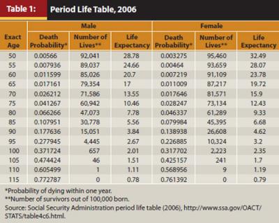
The sustainable withdrawal rate available from a retiree’s portfolio depends on a number of factors. The withdrawal rate itself is a variable that depends directly on time because it changes as the retiree ages—it goes up as the retiree ages or the expected distribution period shortens. Thus, longevity probability is a very important variable when determining proper age-specific distribution periods. Life expectancies in this paper are based on the Social Security Administration’s 2006 periodic life table. Annual changes to the life table have not been material, and therefore should not make a large difference in findings and methodology. However, just as market data may update results over time, periodic life table adjustments should also be applied so that both market and longevity effects are slowly captured in this model over longer periods. For the application of withdrawal rate research in any given country, the expected longevity of that country should be used.
Making decisions based on a single simulation into perpetuity is unrealistic because conditions continually change with time. Proactive or strategic decision making requires a larger context of how a decision to solve one issue (for example, longevity risk) may affect another issue (for example, sequence risk), and may need to include other factors relevant to overall strategic decisions such as asset allocation, time frame, retiree goals, etc.—all of which come from within a model and methodology to evaluate choices. In other words, how do a multitude of possible coexisting transient states relate to each other? Second, models can be developed to compare strategies; for example, different retrenchment strategy models to the baseline model or allocation change strategy models to the baseline model. Last, the methodology should be consistent throughout all models and include the three dimensions of distributions (allocation, withdrawal rate, time) with a focus on probability of failure1 (POF)—a variable that does not depend on time and is therefore a proper variable with which to make key decisions (FMB 2011).
The model and methodology in this paper extend the work of Mitchell (2010 and 2011) and combine Mitchell’s work with the methodology first developed by FMB (2011) to address the following issues simultaneously: (1) applying expected longevity as the distribution period to an age-specific model, (2) evaluating sequence risk as the retiree ages through this model, (3) developing a method to address early on the effect of a retiree continuing to survive beyond longevity estimates, and (4) incorporating decisions for both poor or good market effects (sequence risk). The objective is to develop a more complete model and methodology that address all phases and issues of distributions.
The model developed in this paper will help the reader determine what the effect on withdrawal rate, more importantly POF, is of surviving into the “next” distribution period (DP)—the “next” DP is the then current life expectancy for the then current retiree’s age. The model dynamically adjusts as the retiree ages through rolling distribution periods that decrease slightly in length each year. The authors’ hypothesis is that sequence risk occurs more often and throughout retirement relative to the occurrence of longevity risk; hence the POF-based techniques that manage exposure to sequence risk also simultaneously manage aging into and through superannuation.
The authors’ model no longer shows generic distribution periods. Instead, the current age of the retiree is used as the starting point for each year during simulation. The DP is derived by subtracting the current age from the percentile longevity age (from periodic life tables). Joint couples are assumed to be the same age for concept development purposes. For example, a 65-year-old couple in which either, or both, have a 20 percent chance to live beyond age 95: DP = 95 – 65 = 30 years. This DP calculation is updated annually within the simulation.
The overall effect of using joint data initially is for longer DPs in the model, thus making the model more conservative than would be the case for either single female or single male scenarios. Further model development and research is needed for situations of singles, although the effect would be slightly shorter DPs compared with joint data, thus resulting in slightly higher withdrawal rates. Various age differences within couples would also affect DPs and therefore withdrawal rates.
The authors combine male and female life expectancy statistics and assume independence to determine joint probabilities. For example, if the probability of a 65-year-old male living to age 85 is 40 percent, and the probability of a 65-year-old female living to age 85 is 50 percent, the probability that either or both would live to that age would be 1 minus the probability that both are dead, which would be 70 percent (1 – [(1 – .4) x (1 – .5)]); or alternatively, a 30 percent chance to outlive 85 (Goodman 2002). In this manner, specific ages are combined with specific life expectancies to move away from generic distribution periods. Various thresholds of life expectancy are used in this paper, for example, 75th percentile (75 percent chance of outliving the distribution period), 50th percentile, and 25th percentile, in order to evaluate directly how longevity percentile affects the model.
The use of life expectancy as the current DP as the retirees dynamically age will be discussed below. A data cross section (Table 1) for the DPs is extracted from the latest (2006) Social Security period life table. The model uses the 50th percentile as a proxy for expected longevity.
Asset Classes
Returns are based on five asset classes from January 1926 until December 2010. All returns are converted into “real returns” (adjusted for inflation); inflation is defined as the increase in the Consumer Price Index for All Urban Consumers, from the Bureau of Labor Statistics.
Cash: 30-day T-bill
Bonds: Ibbotson Associates Long-Term Corporate Bond Index
Domestic Large-Cap Equity: S&P 500 Index
Domestic Small-Cap Equity: Ibbotson Associates U.S. Small Stock Index
International Large-Cap Equity: Global Financial Data Global ex USA Index from January 1926 until December 1969 and then the MSCI EAFE from January 1970 until December 2010
Portfolios are constructed of two components: cash/fixed and equity. The cash/fixed component is 25 percent cash and 75 percent bond. The equity component is 50 percent domestic large-cap equity, 25 percent domestic small-cap equity, and 25 percent international large-cap equity. For example, a 60/40 portfolio (60 percent equity and 40 percent cash/fixed) would have 30 percent domestic large-cap equity, 15 percent domestic small-cap equity, 15 percent international large-cap equity, 10 percent cash, and 30 percent bond.
Time Sequencing and Simulation Periods
The authors use a 3D method of graphing to illustrate the dynamic concept of transient states, in which each data point represents a possible withdrawal state for a retiree at that specific point in time, and how that transient state may relate to other possible transient states the retiree may experience given changing market return sequences, retiree withdrawals, and/or asset allocation.
For Phase 1, a 10,000-run Monte Carlo generator was built in Microsoft Excel. The distribution is assumed to be taken from the portfolio at the beginning of each year. All returns are in real terms so that a constant real withdrawal amount is assumed to be taken from the portfolio during each year in retirement. Returns are generated assuming a normal distribution based on the average historical annual real returns and standard deviation, not the actual historical series and not bootstrapped. The success of a portfolio or withdrawal is calculated by determining how many portfolios had positive values at the end of the year. A positive value would indicate the portfolio was successful for that year. Withdrawal rates are tested in .05 percent increments from 0 percent to 25 percent, in .10 percent increments from 25 percent to 50 percent, and in .25 percent increments from 50 percent to 100 percent. The simulation is based on a period dependent on the retiree’s probability of outliving the distribution period as described for Table 1.
Phase 1
Rather than illustrate distribution periods on a figure’s time axis, this paper introduces the retiree’s age on the time axis with each simulation distribution period from the expected longevity for each retiree age from Table 1, resulting in an age-based model.
The model (Figure 1) in this phase most closely represents how advisers envision retirement withdrawals, now in 3D. However, after the distribution period begins, few advisers annually adjust the distribution period dynamically as the retiree ages. The DPs in Figure 1 represent the estimated expected longevity of the retiree (50th longevity percentile). The withdrawal rate at the beginning of each DP represents the starting withdrawal rate for that age-specific DP. The fundamental difference for this paper is the adjustment of the distribution period each year the retiree ages—rolling DPs (decreasing lengths) as the retiree ages each year with a subsequent rolling recalculation of the withdrawal rate; an annual determination of the current transient state. All solutions on the 5 percent POF landscape represent transient states (solutions) with 5 percent or fewer of the simulations failing to reach the end of the DP; similarly for the 50 percent POF. Other POF landscapes exist between 5 percent and 50 percent, illustrated in Figure 2, and represent the range of POFs that coexist (FMB (2011)).
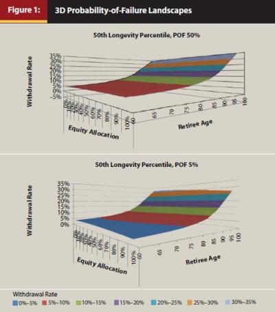
Figure 2 illustrates age (distribution time remaining) cross sections through Figure 1. For example, the same 10 percent POF landscape from Figure 1 has a 4.1 percent withdrawal rate at age 60, a 5.3 percent withdrawal rate at age 70, and an 8.1 percent withdrawal rate at age 80 (all 60 percent equity allocation and 50th percentile longevity expectancy), and transient states coexist for the 30 percent POF landscape, respectively: 5.1 percent at 60, 6.5 percent at 70, and 9.5 percent at age 80.
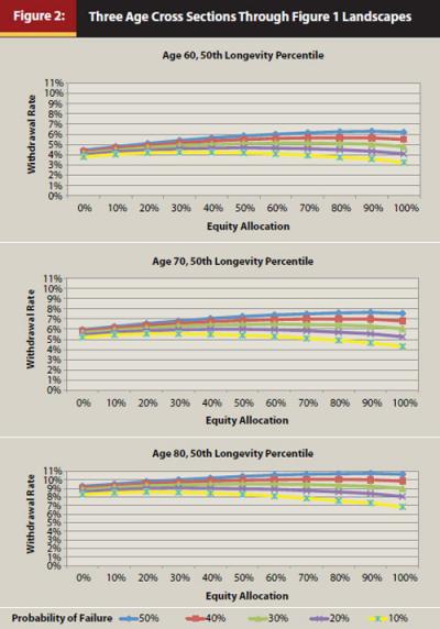
Most advisers think in terms of constant asset allocation and illustrate their figures along the asset allocation plane. The authors show cross sections to demonstrate how the withdrawal rate is actually a time-dependent variable and also show that the time-independent variable is the probability of failure.
POF landscapes would shift the withdrawal rates up (not illustrated) as the longevity percentile increased.2 This occurs because distribution periods are shorter for higher longevity percentiles and longer for lower longevity percentiles. For example, the 75th longevity percentile represents people who outlive a period shorter than expected longevity (50th percentile), and the 25th longevity percentile represents people who outlive a period longer than expected longevity. This withdrawal rate shift, as a result of changing the longevity percentile, will be further explained in Phase 2.
Some Phase 1 observations include:
- Withdrawal rates change naturally as the retiree ages. Thus, a set “safe” withdrawal rate (0 percent POF), for example, 4 percent, is not optimal for all retirees because not all retirees are the same age.
- Dispersion of POF in Figure 2 appears to be a function of volatility in which POF dispersion is “narrow” for lower equity allocations and “wider” for higher equity allocations. This is an area for further research.
- Of interest: the differences between outliving expected longevity percentiles increase as the retiree ages.
The last observation will be the focus of strategy application in Phase 2, in which the longevity percentile variable will also be dynamically altered during simulations.
Phase 2
When the distribution period used is expected longevity, the question then arises: what happens to retiree withdrawal values when the retiree lives beyond expected longevity? Phase 2 seeks to solve this fundamental problem—it is uncertain which retirees in the population will experience superannuation. Clearly, those who are already ill are unlikely to outlive expected longevity. What about those who exhibit no sign of illness? Phase 2 of this project evaluates how the methodology applies to a retiree who continues to “age through” the period life table.
Cash-flow values are expressed in real terms, thus representing the same level of income replacement when factoring in inflation.
Klinger (2007, 2010) researches higher withdrawal rates early in retirement and reduces them later in retirement, and he suggests a method to do this. This paper develops a method to reduce withdrawal rates through evaluating the percentage who may outlive expected longevity. The methodology uses DPs based on the length of lifetimes as adjusted by a dynamic change to the percentage of the population expected to outlive expected longevity. The effect is to shorten the DPs, thus increasing withdrawal rates relative to static DPs, and provide a rational method to assign DPs to specific retiree ages. The result: an age-based model that also allows for differences between retiree goals of early consumption versus later consumption (inheritance).
General Initial Reflections
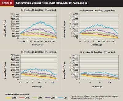
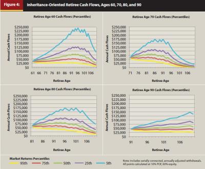
Figures 3 and 4 reflect serially connected, annually calculated cash-flow percentiles as cash-flow snapshots of a retiree aging and use the longevity percentile expectation to establish the length of the DP. This process determines an optimal withdrawal rate for that specific annual transient state, based on setting the expected POF at 10 percent. The resulting withdrawal rate is the same across all cash-flow percentiles at each age; for example, 4.65 percent (Figure 3) or 3.60 percent (Figure 4), both at age 62—thus withdrawal rates are directly sensitive to the longevity-percentile-calculated DP. What changes is the portfolio value based on “good” or “bad” simulated markets. The 5th (best one in twenty) and 25th (best one in four) percentiles represent the “good” market sequence cash flows and the 75th (worst one of four) and 95th (worst one of twenty) percentiles represent the “bad” market sequence cash flows, all from different annual starting portfolio values (transient states). Note that a retiree may experience “good” markets and be above the 50th percentile during one period (age 60 simulation) and experience “bad” markets and be below the 50th percentile during another period (age 62, or any subsequent age simulation) because sequence risk is ever-present during retirement.
The tendency is to look at graphs or calculations as “prophetic.” Observe that at age 61, for example, it is not certain at age 70 how the markets may have performed in the interim. Only at age 70 can the transient state for a 70-year-old be assessed.
There are corresponding portfolio values that support their respective annual percentile cash flows. Note that there are now two sets of percentiles: one for longevity (to determine distribution periods) and another for different possible market sequences.
FMB (2011) demonstrates how using POF in a 3D model assists in evaluating exposure to sequence risk. It also helps determine when to make a decision about changing the withdrawal amount by allowing POF to float as a result of the withdrawal rate changes because of market returns, before either a retrenchment (bad market) or additional spending (good market) decision is made. A single asset allocation (60 percent) was used for Figures 3 and 4; however, similar results emerge with any other allocation with differences only in cash-flow amounts and general trends in percentiles because of allocations expected from heavier bond or equity exposures.
Consumption-Oriented Retiree
A “consumption-oriented” retiree can be demonstrated through the interaction and utility of longevity percentile to determine the starting DP variable. Retirement should be viewed as a dynamic rather than set-and-forget exercise. The DP for expecting 75 percent of the retirees to outlive the time horizon results in a higher withdrawal rate because the DP is shorter relative to the 50th longevity percentile, which is shorter relative to the 25th longevity percentile. The shorter DP results in a higher possible relative withdrawal rate, all within the same POF landscape.
As the retiree ages in Figure 3, the longevity percentile (longevity “lever”) is reduced periodically (every five years in this model), thus dynamically extending the DP. For example, a 60-year-old retiree may start with the 75th longevity percentile, then adjust to 65th percentile at age 65, 55th at age 70, 50th at 75, 40th at 80, 30th at 85, 20th at 90, and 10th at 95 and beyond. This scenario reflects reality in that the 75th percentile is not used throughout the simulation, but instead for a brief period. Cash flows are calculated annually and the withdrawal rate is adjusted annually based on the annually recalculated DP, with all simulations constrained to have 10 percent or fewer fail to reach the end of that current year’s DP.
This is a dynamic, serially connected, annual rolling adjustment that slowly extends the DP so the retiree has a smaller probability of outliving the DP from his or her current retirement age when the transient state is re-evaluated. This model is thus a longevity-based methodology that investigates how to achieve Klinger’s objective in which retirees begin with a higher withdrawal rate and adjust the withdrawal rate as they age. Also note that the longevity percentile reduction is an example for concept demonstration purposes and not represented as an optimal solution.
Consumption-oriented retirees may find they are “unlucky” and experience market returns under the 50th market returns percentile (Figure 3). These retirees would need to adjust their withdrawal dollar amounts down. Alternatively, a retiree may choose lower longevity percentile values, the impact of which will be to extend the DP, thus reducing the withdrawal rate with the same target POF. The opposite would apply to a “lucky” retiree who experiences better than 50th market returns percentiles. Market returns do not separate retirees by the year they retire; rather, the POF function is best used as a method to evaluate exposure to market returns sequence risk based on FMB (2011)—when POF increases, the withdrawal dollar amount should be adjusted to reduce the probability of exhausting the portfolio within the current DP (retrenchment), and vice versa if POF decreases.
Alternatively, retirees may choose to be more conservative from the beginning of retirement so that more of their portfolio value extends into their later years. This is accomplished by using low longevity percentile values (for example, the 10th longevity percentile) to determine the DP. The authors label such a retiree “inheritance oriented,” which is illustrated in Figure 4.
Inheritance-Oriented Retiree
Figure 4 illustrates a low, constant 10th longevity percentile across all ages for an “inheritance-oriented” retiree. Note that the cash flows are shifted toward later retirement ages as compared with those of the consumption-oriented retiree. The use of longevity percentiles allows the practitioner to measure and manage either “pulling” retirement consumption into early years or “pushing” retirement consumption into later years—or the ability to switch between either goal at any time. This pull or push is visualized by comparing the retiree age at which the “hump” occurs between Figures 3 and 4.
Phase 2 combined uncertain market returns (probability of the portfolio) with uncertain longevity (probability of the person) into one age-based distribution model for goals of consumption or inheritance that is also three dimensional when asset allocation and POF are incorporated, as demonstrated in Phase 1. Some Phase 2 observations include:
- Using higher longevity percentile values (shorter DPs early on), and moving toward lower values as the retiree ages (longer DPs later), tends to maximize the retiree income over the retiree’s lifetime. This is an example of using longevity percentile values for a consumption-oriented retiree described in Figure 3. The longevity percentile values are for concept demonstration of polar retiree strategies, not necessarily suggested values.
- Frank and Blanchett (2010) found that exposure to sequence risk never goes away. The results from the methodology in this paper support this observation—percentile ranges at all ages had either “good” or “bad” cash-flow values regardless of the retiree’s age (percentile “bow waves” in Figures 3 and 4. Bow waves are discussed below in the Sequence Risk section).
- The later retirement age cash flows decline primarily because of the effect of ever-shorter DPs as a result of fewer years of life expectancy. Further research should look specifically at developing methods to evaluate later-age (superannuation) cash-flow strategies according to retiree goal (consumption versus inheritance).
- Possible insight into further superannuation strategies comes from Mitchell (2010), who demonstrates that the uncertainty of remaining life span increases as the retiree ages even though there is a reduction in the number of expected remaining years.
Sequence Risk
How does sequence risk, with subsequent adjustment to the withdrawal amount, affect the distributions for retirees who continue to live beyond expected longevity?
Because withdrawal rates naturally increase for retirees as they age as a result of a decreasing DP, it is difficult to separate out an increasing withdrawal rate because of the aging effect from a bad market sequence effect. The withdrawal rate also is affected to some degree by asset allocation. Because market values change more rapidly relative to aging, the sequence risk effect is observed more often.
The bow wave in Figures 3 and 4, which emanates and widens from each simulation starting age, illustrates sequence risk and represents the possible distribution of unknown outcomes that exist at any simulation’s starting age. For example, the illustration for the 71-year-old is simply one possible sample of what a 61-year-old retiree may experience when he or she reaches age 71. It remains unknown just where market sequences may take a retiree, even for the subsequent year. These cash-flow percentiles represent transient states that may be monitored through POF, and decisions can then be made, according to FMB (2011), to reduce the dollar amount withdrawn as POF approaches or exceeds 30 percent.
Overall Conclusions
The development of an age-based model is more meaningful than generic distribution period analysis because an age-based model incorporates life expectancy uncertainty in addition to market uncertainty. This paper demonstrates a methodology to unify into a single model the various factors that affect decumulation.
- The concept of transient states suggests that the retiree’s decumulation goes through a dynamic process of change over time and market changes. A retiree moves between the POF landscapes with every market move and every change in time. The simulation that tells us where the retiree is within the landscapes is associated with conditions in that brief moment (transient state). Redo the simulation again at a later time with a different portfolio value, and you arrive at a different place in the landscapes. Many of the transient states are okay. As they approach the 30 percent POF boundary (because of poor markets or large lump-sum withdrawal, FMB 2011), then a decision should be made to pull them away from that boundary. As they move away from that boundary they are better off (good markets). Pulling them away from a high POF boundary may be accomplished by reducing the withdrawal dollar amount or reducing the longevity percentile value.
- The transient state perspective leads to serially connected, constantly adjusting annual distribution periods rather than a disconnected fixed distribution period based on no determinable end point.
- The DP may be dynamically managed as the retiree ages by varying the percentage who outlive expected longevity (longevity percentile). Shorter DPs result in higher withdrawal rates, and by evaluation of the longevity percentile, DP lengths may change dynamically. Longevity percentile is a useful “lever” to manage distribution periods.
- Mitchell (2010) demonstrates that the uncertainty of remaining life span increases as the retiree ages even though there is a reduction in the number of expected remaining years. Both consumption- and inheritance-oriented retirees experience decreasing cash flow in the superannuated years as a result of the higher withdrawal rates associated with short DPs corresponding to very short expected longevity. This is a future area of research.
The withdrawal rate is a poor metric for retirement success because it is sensitive to DP as well as market returns on portfolio values. The DP is not a fixed period—it may be changed dynamically as the retiree ages by changing the longevity percentile for the retiree’s current age. The longevity percentile is also not a fixed value; it too may be changed. The POF is best used as a measure of exposure to market sequence risk. This paper, combined with FMB (2011), demonstrates that withdrawal rate is a dynamic function of other variables, including portfolio allocation, each of which should be evaluated three dimensionally in relation to each other to access the current transient state of a retiree during decumulation years.
Researchers have sought a single “safe” withdrawal rate that would last the retiree from retirement to death. The dynamic model in this paper, combined with the authors’ prior paper, however, develops a methodology to monitor, evaluate, and react as necessary to transient states as well as base the model on age-specific expected longevity rather than generic, ageless, or unanchored distribution periods.
Two sustainable ranges of withdrawal rates exist: the first is based on the longevity percentiles’ effect on DP bounded by consumption (upper range) or inheritance (lower range) goals; the second is determined within the first’s DP based on market fluctuation effects on portfolio values bounded by high POF/high withdrawal rate (upper range because of “bad” sequence) or low POF/low withdrawal rate (lower range because of “good” sequence).
The methodology presented here provides a model to directly incorporate longevity risk and provides a rational alternative to guarantees, implemented here through index funds, with the option to switch to a guarantee at any later time. A dynamic model provides more assurance that retirees may be able to maximize their cash distributions over their lifetimes. Modifying longevity statistics for health reasons is problematic unless reliable statistics are available for a client’s specific health condition. This paper provides a conceptual methodology to better assess where a retiree may be found in a distribution model that incorporates longevity statistics directly to determine distribution periods.
Practical Application
Practitioners can apply two components of this paper while software developers consider and catch up with the methodology studied here. Until software directly applies longevity percentiles to determine DP lengths, practitioners should access longevity tables for expected longevity (50th percentile) ages, and adjust that age to then determine the current DP. From a transient state perspective, the DP would apply to the retiree’s current age for the current DP and would be readjusted in subsequent years when simulations are rerun. After the DP has been calculated, the current software available to practitioners may be used to determine the current POF.
Note the tendency to interpret figures and calculations as being predictive. The figures here illustrate that the future is unknown. People do not know whether they will be in the 75th percentile or 25th percentile, or any other possible percentile. The current transient state and trend is determined through evaluation of the current POF. If the POF is rising, for example from 10 percent to 15 percent, this is an indication of an increased probability that the current withdrawals may not be sustainable. From FMB (2011), the retiree can pre-calculate and consider a change of the withdrawal dollar amount to reduce the POF, then adjust back to a more successful track. This adjustment is still not predictive because we do not know what track will result from future markets. Thus, the concept demonstrated here is a transient model that uses both probabilities of the portfolio and probabilities of longevity, combined with the FMB (2011) probability-of-failure evaluation, as a more comprehensive model for retiree distributions.
Endnotes
- Probability of failure (POF) comes from prior conventional use of the term. Percentage of failure would be more accurate because the results represent the percentage of simulations that do not reach the end of the simulation period in question.
- A working paper, which includes appendices with data that demonstrate how these figures are developed, and additional data, is available at SSRN: www.ssrn.com/abstract=1849983.
References
Frank, L. R., and D. M. Blanchett. 2010. “The Dynamic Implications of Sequence Risk on a Distribution Portfolio.” Journal of Financial Planning 23: 52–61.
Frank, L. R., J. B. Mitchell, and D. M. Blanchett. 2011. “Probability-of-Failure-Based Decision Rules to Manage Sequence Risk in Retirement.” Journal of Financial Planning 24: 46–55.
Goodman, Marina. 2002. “Applications of Actuarial Math to Financial Planning.” Journal of Financial Planning (September).
Klinger, W. 2007. “Using Decision Rules to Create Retirement Withdrawal Profiles.” Journal of Financial Planning 20: 60–67.
Klinger, W. 2010. “Creating Safe, Aggressive Retirement Income Profiles.” Journal of Financial Planning 23: 44–53.
Mitchell, J. B. 2010. “A Modified Life Expectancy Approach to Withdrawal Rate Management.” Presented at Academy of Financial Services, Denver, Colorado. www.ssrn.com/abstract=1703948.
Mitchell, J. B. 2011. “Withdrawal Rate Strategies for Retirement Portfolios: Preventive Reductions and Risk Management.” Financial Services Review 20: 45–59.