Journal of Financial Planning; March 2012
Jerry A. Miccolis, CFA, CFP®, FCAS (miccolis@brintoneaton.com), is a principal and the chief investment officer at Brinton Eaton, a wealth management firm in Madison, New Jersey, as well as a portfolio manager for The Giralda Fund. He co-wrote Asset Allocation For Dummies® (Wiley 2009), and numerous works on enterprise risk management.
Marina Goodman, CFP® (goodman@brintoneaton.com), is an investment strategist at Brinton Eaton and a portfolio manager for The Giralda Fund. She has been working to bridge the gap between research and practice in improving the portfolio optimization process.
At the heart of portfolio diversification is the assumption that at least some assets have low correlations with each other. Underestimating correlation leads to overestimating the portfolio’s true diversification. This becomes particularly dangerous during times of market stress, when contagion sets in and the investment adviser gets caught by surprise at how much the assets begin moving together—and in the wrong direction!
Having a better understanding of how assets relate to each other dynamically across different environments can help the adviser build a truly diversified portfolio and help identify the times when the portfolio may be most vulnerable.
Most people think of correlation as a single number; however, a single number cannot capture the dynamic nature of correlation. Here we explore various ways of viewing the relationship between assets in a more comprehensive way.
Market Forces
One reason for a dynamic approach to correlation is that correlations can change as fundamental market forces change. A useful way to capture these changes is to calculate rolling correlations over a certain period, such as three years, which is long enough to observe a stable pattern and short enough to be timely. An example is the rising correlation between domestic and international equities resulting from the increase in globalization (the blue line in Figure 1)—a change that occurred gradually and, some would say, predictably.
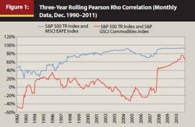
An example of a sudden and unexpected change is the increase in the correlation between commodities and equities (the red line in). This phenomenon started with contagion in the fourth quarter of 2008 and has continued, perhaps because of greater investor access to commodities and the emerging prominence of the “risk on/risk off” mentality affecting virtually all types of risky assets.
Correlations that change over time are more the rule than the exception, so a measurement over any historical period may not be relevant to the period over which your portfolio needs to perform. Failure to reflect that fact may result in portfolios that are much more dangerous than you think.
Asset Behavior
There are more troubling problems with traditional measures of correlation. A particularly grievous one is that, in addition to being time-dependent, correlations are dependent on how well the assets themselves are behaving. One way to view this phenomenon is via a scatter plot in which the returns of one asset are graphed along the x-axis and the returns of the other asset are graphed along the y-axis. Each point on the graph represents the return for each asset in a particular common month. In Figure 2, we compare the monthly return of the S&P GSCI commodity index with the monthly return of a long/short commodities momentum strategy, the Commodities Trends Indicator (CTI), available to the retail investor through several investment vehicles. This scatter-plot view allows one to immediately see the return distributions for both asset classes.
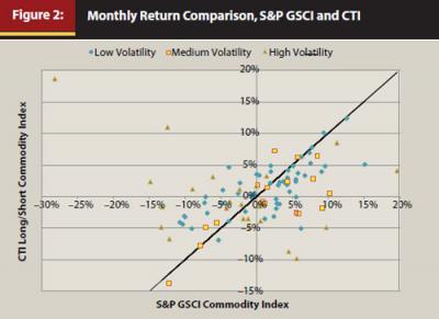
The black line indicates where the CTI return would lie if it equaled the commodities return each month. This line helps us to easily identify months when CTI outperformed commodities (being above the black line) or underperformed (being below the black line).
Figure 2 shows more interesting behavior than what a single correlation number could hope to capture. For example, when the returns on commodities are positive, the CTI tends to underperform. However, when returns on commodities are negative, the CTI usually outperforms—and the more negative the commodity returns, the more likely the CTI will outperform and the greater the degree of outperformance. This makes a much stronger argument that these strategies are good diversifiers to each other than a simple correlation measurement—or even a rolling correlation picture—would imply.
This example points out an oft-ignored feature of traditional correlation coefficients—they measure the degree to which the relationship between two things is linear; they are baffled by non-linear relationships, of which there are many in the real world. Figure 2 shows how this scatter-plot tool can be particularly useful in evaluating alternative investments, which often have unique and non-linear relationships with more traditional assets and strategies.
Time and Other Criteria
The scatter plot shown does not include the dimension of time, so you can’t tell if a particular data point was recent or from years ago. It can therefore mask changing correlations over time. One way to include time is by making the returns from each period a distinct data series and using a unique color for each. This enhanced view can convey much the same information as the rolling-correlation view shown in Figure 1.
Taking this idea a step further, the return history can be parsed based on any criteria one chooses. An adviser can develop a taxonomy of different market environments based on some economic or market criteria, for instance. This tool can then help the adviser refine the assumptions—on expected return, risk, and relationships between assets that go into an asset allocation optimization model—to reflect the projected market environment.
For example, what if the returns were color-coded (and/or shape-coded) based on the average level of volatility (VIX) for that month? You can see that adding this feature in Figure 2 helps vividly show how the assets perform in a low-, medium-, and high-volatility environment. The adviser can now make a direct link between the kind of volatility regime he or she thinks is most likely and the resulting returns, risk, and correlations for the asset classes under review.
Having a comprehensive understanding of the true relationships between assets is key to building a well-diversified, robust portfolio. Any correlation measure that presumes these relationships are static, linear, and unaffected by the market environment is unlikely to help the adviser reach that level of understanding.