Journal of Financial Planning: June 2019
John T. Scruggs, Ph.D., is the former vice president of research at Loring Ward in San Jose, California. Previously, he also served as a research officer in the quantitative equity and index businesses at BlackRock as well as a finance professor at the University of Georgia and Washington University in St. Louis. His areas of expertise include quantitative investment management, empirical asset pricing, risk modeling, and financial econometrics. His research has been published in various journals, including the Journal of Finance and the Journal of Financial and Quantitative Analysis.
Executive Summary
- This paper demonstrates how moving three choice levers (asset allocation, initial withdrawal rate, and withdrawal flexibility) affects the joint distribution of retirement outcomes in terms of future consumption and terminal wealth.
- Using Monte Carlo simulation, the joint effects of the three choices on retirement outcomes in terms of income and terminal wealth were investigated.
- Results indicate that withdrawal flexibility effectively transferred some portfolio risk from a household’s wealth to its income, and allowing for even modest withdrawal flexibility dramatically reduced the probability of running out of money.
- Because retiree goals in terms of lifestyle and legacy can be related to income and terminal wealth, a case may be made for featuring regular Monte Carlo simulation in the retiree decision-making process.
Acknowledgment: The author acknowledges contributions by Jim Davis, Larry Frank, Jim Healy, Sam Savage, Manish Singh, Meir Statman, colleagues at Loring Ward (which funded this research), and seminar participants at the 2018 ProbabilityManagment.org conference, where this research was first presented.
Aside from luck, investment outcomes for newly retired households are largely determined by three key choices: asset allocation, initial withdrawal rate, and withdrawal flexibility. These choices can be thought of as the three levers with which retirees can exert some control over the distribution of retirement outcomes in terms of future consumption and terminal wealth.
Choices naturally involve trade-offs. Asset allocation choices involve the trade-off between risk and expected return. Choosing high withdrawal rates or requiring excessively smooth consumption can prematurely deplete wealth. All else equal, lower withdrawal rates result in higher terminal wealth. The choices retirees make to resolve these trade-offs are highly idiosyncratic. Households have different preferences, circumstances, and goals. It follows that no set of choices is optimal for all households. The goal of this paper is to provide some insights into how retiree choices affect the joint distribution of retirement outcomes.
Literature Review
Early research in this area focused on a common question posed by retirees to their financial advisers: “How much can I afford to withdraw each year?” The question remains important. It affects not only the household’s lifestyle, but whether that lifestyle can be sustained in the long run. The Association of International Certified Public Accountants (AICPA) reported that “running out of money” and “maintaining their current lifestyle and spending level” were the top two retirement planning concerns for their clients in a 2016 survey.1
Seminal research produced an enduring rule of thumb: the 4 percent rule (Bengen 1994, 1996; and Cooley, Hubbard, and Walz 1998) in which a newly retired household takes 4 percent of their portfolio value as a withdrawal in the first year of retirement. Thereafter, they withdraw the same inflation-adjusted (or real dollar) amount every year. Cooley, Hubbard, and Walz (1998) found that a portfolio with a significant equity allocation (50 percent or more allocated to common stocks, the remainder to long-term corporate bonds) had a probability of success (defined as not running out of money) greater than 95 percent for a 30-year horizon.
The 4 percent rule is a constant real dollar spending rule. Constant real dollar spending rules are inflexible withdrawal strategies; they make no adjustment for future investment performance. In an inflexible withdrawal strategy, one of the choice levers is effectively stuck.
More recent research has found that introducing withdrawal flexibility can substantially increase the probability of success or permit higher initial withdrawal rates. Various research papers have devised “decision rule” methods for determining dynamic withdrawals.
Bengen (2001) proposed a constant fraction rule with ceilings and floors on real withdrawal levels. Jaconetti, Kinniry, and DiJoseph (2013) proposed a constant fraction rule with floors and ceilings on changes in real withdrawals. Guyton and Klinger (2006) proposed a complex set of rules governing how real withdrawals are changed, conditional on portfolio performance, initial spending rates, and the remaining planning horizon. Zolt (2013) proposed a glide path rule cognizant of both past consumption and capital requirements for future spending. The rule provides cost-of-living adjustments to spending only when wealth is sufficient to support future planned spending; real withdrawals are never increased; and nominal withdrawals are never reduced.
A chapter in Pfau (2017) is devoted to dynamic withdrawal strategies and their role in managing sequence risk. Using a fixed stock/bond allocation and a common set of assumptions, Pfau evaluated 10 decision rules and compared the distributions of real spending and terminal real wealth.
This paper examined the effects of varying the three choices of asset allocation, initial withdrawal rate, and withdrawal flexibility on the joint distribution of retirement outcomes in terms of real consumption and terminal real wealth. Particular attention was paid to the effects of moving the withdrawal flexibility choice lever while remaining agnostic regarding an optimal set of choices or outcomes. This paper did not attempt to evaluate the efficacy of existing rules. Any such evaluation would require specifying a utility function (e.g., Blanchett 2017) or scoring metrics (Pfau 2015, 2017).
Varying the Withdrawal Flexibility Lever
Varying the asset allocation or initial withdrawal rate levers is straightforward. Varying the withdrawal flexibility lever requires a mechanism for precisely controlling the degree of consumption smoothness in an experimental setting. The hybrid approach of Jaconetti, Kinniry, and DiJoseph (2013) served this purpose. At one extreme of the hybrid continuum are inflexible withdrawal strategies such as the 4 percent rule. At the other extreme, a constant fraction spending rule is an infinitely flexible withdrawal strategy.
Under a constant fraction spending rule, the level of the nominal withdrawal is determined by multiplying the portfolio balance by the chosen fraction. Changes in the level of real withdrawals mirror changes in the inflation-adjusted portfolio balance. The withdrawals could become vanishingly small. Yet, a constant fraction spending rule virtually assures “success.”2 In a twist on Zeno’s dichotomy paradox, an infinite number of constant fraction withdrawals would never exhaust a portfolio’s value. Therefore, a flexible withdrawal strategy might mollify a household’s concerns about running out of money, but it would do little to reassure them about the sustainability of their lifestyle.
Neither the constant real dollar nor constant fraction withdrawal strategies may be realistic choices for retirees. On the one hand, households have a natural inclination to reduce discretionary spending in the wake of market downturns. It is unrealistic to assume that households will stick to a constant real dollar spending rule in the face of dwindling assets. After the global financial crisis, the IRS was pressured to suspend the required minimum distribution requirement for 2009 (IRS Notice 2009-09). Yet, many planning software programs employ an inflexible withdrawal strategy in Monte Carlo simulation of future outcomes.
On the other hand, the highly volatile consumption growth associated with a constant fraction withdrawal strategy is unlikely to be palatable for a household with relatively fixed expenses or tastes. Households care about the smoothness of their consumption over time. Modeling preferences for consumption smoothness has long been a feature of intertemporal asset pricing literature. For example, the time-separable utility function of Epstein and Zin (1989, 1991) featured two preference parameters: the familiar coefficient of relative risk aversion, and the elasticity of intertemporal substitution. If smoothness of consumption growth is a matter of household preference, then one could argue it should be modeled in Monte Carlo simulation.
If neither of the extreme withdrawal strategies are realistic for retirees, then it is important to understand how moving the withdrawal flexibility lever affects attainment of retiree goals. Retiree goals can be expressed in terms of lifestyle and legacy. Lifestyle goals can be related to future retirement income. Legacy goals can be related to terminal wealth. In making choices, households implicitly make trade-offs between these goals.
Experimental Design
Consider a meeting between a financial planner and a newly retired household. The household has $1 million in investable assets and a planning horizon of 30 years. The household desires to take a cash withdrawal immediately and further withdrawals annually thereafter for 30 years (for a total of 31 withdrawals). The household must choose an asset allocation for their investable assets, a withdrawal strategy with an initial withdrawal rate, and a level of withdrawal flexibility. Therefore, the household has three choices (or levers) with which to affect its retirement outcomes. The experiment examined in this paper considered 198 permutations of those three choices (six equity allocations x three initial withdrawal rates x 11 withdrawal flexibility levels).
Asset allocation—the first lever. For simplicity, two assets (equity and cash) and six equity allocations (0 percent, 20 percent, 40 percent, 60 percent, 80 percent, and 100 percent) were considered. Rather than employ historical returns, it was assumed that real asset returns were independent and identically distributed multivariate normal, given the capital market assumptions reported in Table 1.

Notably, the equity risk premium was assumed to be 6.25 percent per annum—considerably lower than the equity risk premium implicitly implied by other studies that employed historical data. However, it is consistent with academic research suggesting that the equity risk premium has declined (Fama and French 2002). For purposes of the experiment, the key assumption was that portfolio risk and expected return were increasing in the portfolio’s equity allocation. This paper’s main results would hold for any capital market assumptions with a reasonable market risk premium. Portfolios were rebalanced annually after the withdrawal was taken.
Withdrawal strategy—two more levers. The withdrawal strategy provided two more levers to households: the initial withdrawal rate and the level of withdrawal flexibility. The initial withdrawal rate operated as in a constant fraction withdrawal rule. The rate was simply applied to a portfolio’s ending balance to determine the amount of the cash withdrawal. The experiment considered three initial withdrawal rates: 3.5 percent, 4 percent, and 4.5 percent.
The final lever was withdrawal flexibility. The desired level of consumption smoothness was achieved by choosing a limit on the magnitude of the absolute percentage changes in inflation-adjusted withdrawals. The absolute percentage limits were applied to the change in withdrawal from the previous year. Eleven withdrawal flexibility levels were considered: 0 percent to 5 percent in 0.5 percent increments.
For purposes of this paper, the limits were symmetric. However, there is no need for the limits to be symmetric in practice. Higher limits represent more withdrawal flexibility. Note that a 4 percent initial withdrawal rate coupled with 0 percent withdrawal flexibility delivered the familiar 4 percent rule, which served as the benchmark for comparison in the analysis that follows. This withdrawal strategy is based on Jaconetti, Kinniry, and DiJoseph (2013), which Pfau (2017) referred to as “Vanguard’s Percentage Floor-and-Ceiling Approach.” The salient feature of the strategy was the investor’s ability to choose the desired level of consumption smoothness.
Example of how a withdrawal strategy would work in practice. Assume the household with a $1 million portfolio chooses an initial withdrawal rate of 4 percent and withdrawal flexibility of 2 percent. Table 2 demonstrates how withdrawals would be computed given portfolio returns of –6 percent, +10 percent, and +10 percent in the first three years of retirement. At times 1 and 2 (as shown in Table 2), the 2 percent withdrawal flexibility parameter is binding on the down side. At time 3, it is binding on the up side.

Unmodeled features. It is not the purpose of this paper to recommend an optimum set of decisions for retired households. Rather, this paper examined the effects of varying the three choices (asset allocation, initial withdrawal rate, and withdrawal flexibility) on the joint distribution of retirement outcomes in terms of real consumption and terminal real wealth. It is not the retirement outcomes themselves that matter, but the differences between retirement outcomes that arise when choices are perturbed. Therefore, for purposes of analytical tractability, this study ignored several potentially important aspects of retirement investment decisions—the most obvious being longevity risk.
Uncertainty about lifespans is a first-order concern for retired households. It is unrealistic to assume a horizon of 30 years is appropriate for all households. However, the 30-year horizon has been a fixture in the literature since Bengen (1994), and results based on a fixed 30-year horizon are useful for comparison. The relation between dynamic withdrawal rates and decreasing remaining life span is briefly discussed in a later section.
This paper makes no judgements regarding the household’s willingness or ability to withstand decreases in real consumption. Presumably, a household would consider these factors when making its choices. Likewise, pension income, annuity income, or consumption flows from durable assets such as housing were ignored in this analysis. Blanchett (2017) found that guaranteed income had a significant impact on safe withdrawal rates. In practice, Monte
Carlo simulation tools would incorporate such flows.
This analysis also ignored taxes and transaction costs. All withdrawals, portfolio values, and returns are expressed in real, or inflation-adjusted, terms.
Simulation Methodology
Ten thousand simulated annual asset return pairs were generated from the assumed bivariate normal distribution. These represent the universe of possible asset returns. For each of the 198 choice permutations, a Monte Carlo trial consisted of 30 years of randomly drawn asset returns. For each Monte Carlo trial, the portfolio was rebalanced annually after the selected withdrawal strategy logic was applied, and 30 years of withdrawals (and a portfolio terminal value) were computed and retained for further analysis. One thousand Monte Carlo trials were simulated for each permutation.
For a Monte Carlo simulation to inform an investor’s choices, the simulated outcomes must be relatable to investor goals. Household goals are typically stated in terms of lifestyle and/or bequest. For households accustomed to balancing a budget, lifestyle goals are readily relatable to a stream of future, inflation-adjusted withdrawals. Bequest goals, whether for heirs or for charities, are relatable to inflation-adjusted terminal wealth. In practice, visual representation of Monte Carlo outcomes is often employed to assess the effects of changes in investment choices. For the purposes of this paper, which compared 198 choice permutations, it was not practical to employ a visual representation of outcomes. Rather, it was necessary to use sample statistics to describe and compare the distribution of retirement outcomes.
It is important to note that the joint distribution of retirement outcomes from a Monte Carlo simulation is conditional on the inputs: initial data and choices. This conditional joint distribution is not static; it changes over time in response to the realization of asset returns and the diminishing number remaining periods. In the absence of mean reversion, below-average portfolio returns will tend to increase the probability of failure for a given withdrawal strategy. Above-average portfolio returns have the opposite effect.3 Holding all else constant, the passage of time will decrease the range of possible outcomes. For clients to know where they stand, Monte Carlo simulation should be periodically repeated with updated inputs. This does not suggest that clients should change their withdrawal strategy. But they should be aware of how the range of outcomes has changed. Dynamic withdrawal strategies can mitigate, but not eliminate, sequence risk.
For terminal wealth, the analysis was straightforward. For each choice permutation, each of the 1,000 sample paths produced a single data point: terminal real wealth. Three sample statistics were employed to describe the distribution of terminal real wealth outcomes: (1) median terminal real wealth (scaled by initial wealth); (2) terminal real wealth volatility (standard deviation scaled by initial wealth); and (3) probability of failure (the fraction of sample paths that had zero wealth at year 30).
For withdrawals, the analysis required two stages. Each Monte Carlo trial produced 31 real withdrawals. Because simulated returns were real, portfolio values and withdrawals were inflation-adjusted by construction. In the first stage, statistics describing the growth rate and volatility of real withdrawals were computed for each of the 1,000 Monte Carlo trials. These first-stage statistics characterized the retirement consumption outcomes for a single trial. In the second stage, statistics summarizing the expected growth and smoothness of real withdrawals, averaged over the trials, were computed for a given choice permutation.
The following statistics describe the distribution of possible retirement consumption outcomes: (1) mean of mean real withdrawal growth; (2) mean of median real withdrawal growth; and (3) mean of real withdrawal mean absolute deviation (MAD).
Two measures of average withdrawal growth rates (mean and median) were examined due to the differing effects of outliers. Large, one-time withdrawal changes occur when a retirement portfolio runs out of money. These withdrawal change outliers can have a substantial impact on the mean growth rate, but have little effect on the median growth rate. Examining both measures of average withdrawal growth provided a more complete picture. The MAD statistic is the mean absolute withdrawal change in percent; it is a measure the “smoothness” of the stream of withdrawals for a given trial. The mean of MAD statistics describe the expected smoothness of income for a given withdrawal strategy.
Retirement Outcomes with Inflexible Withdrawal Strategies
To establish a baseline for comparison, retirement outcomes under the classic 4 percent rule (4 percent initial withdrawal rate, 0 percent withdrawal flexibility) are a useful starting point. Under an inflexible withdrawal strategy, real withdrawals are constant until they’re not. The distribution of real withdrawal changes has significant mass at 0 percent. Negative values only occur for the years in which a portfolio runs out of money (an absorbing state) and are 0 percent again thereafter. Comparing distributions of real withdrawal changes is not very informative when the withdrawal strategy is inflexible. So, this section will focus on how investor choices affect terminal wealth outcomes.
For a given initial withdrawal rate, increasing a portfolio’s equity allocation increases both the median and volatility (standard deviation) of terminal real wealth. This reflects the positive relation between portfolio risk and expected return. Figure 1 depicts how investor choices jointly affect median terminal real wealth and probability of failure. For higher equity allocations, a clear, positive relation exists between initial withdrawal rate and probability of failure. For a given initial equity allocation, spending more increases the probability of failure and reduces expected terminal real wealth. In other words, spending more on lifestyle goals leaves less (perhaps nothing) for bequest goals.
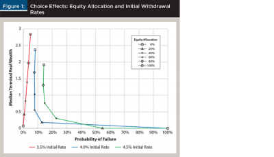
For an all-cash (0 percent equity) allocation, choosing a more conservative 3.5 percent initial withdrawal rate reduces the probability of failure to 0 percent. However, for 4 percent and 4.5 percent initial withdrawal rates, the probability of failure increases to 100 percent. This is because an all-cash allocation does not generate sufficient growth to support higher spending levels.
Retirement Outcomes with Flexible Withdrawal Strategies
The previous section examined how manipulating two levers affects retirement outcomes. In this section, a third lever is introduced. Can households improve their retirement outcomes by employing a flexible withdrawal strategy? What are the joint effects of manipulating the three levers?
The withdrawal flexibility lever, as implemented, was effective; it worked precisely as designed. Figure 2 depicts how the choice of withdrawal flexibility affected real withdrawal volatility (as measured by the mean of real withdrawal MAD) for a 4 percent initial withdrawal rate. For each equity allocation, real withdrawal volatility increased monotonically with the level of withdrawal flexibility. For higher equity allocations, the relations appeared linear with a nearly one-to-one ratio between withdrawal flexibility (a choice) and withdrawal volatility (an outcome).
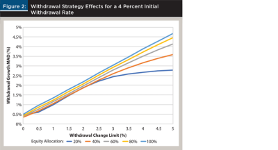
For inflexible withdrawal strategies (those with 0 percent withdrawal change limits) withdrawal volatility was nearly zero. It was entirely driven by trials that ended in failure. Withdrawals drop precipitously when a portfolio runs out of money and remain stable (albeit zero) thereafter. Withdrawal flexibility affects withdrawal volatility, because when withdrawal change limits are increased, withdrawal volatility increases monotonically.
Two things are happening in Figure 2. First, the probability of failure declines as flexibility increases. This reduces the number of precipitous and uncontrollable withdrawal changes, which tends to reduce withdrawal volatility. The dominant effect, however, is controlling the degree to which portfolio risk can be expressed in real withdrawal volatility. For an all-equity portfolio, which has ex ante return volatility of 15 percent per annum, even the highest withdrawal flexibility choice (a 5 percent limit) is binding much of the time. Hence, the real withdrawal MAD is nearly 5 percent.
In fact, there was a direct relation between the withdrawal limit and real withdrawal MAD. When the real withdrawal change limit was fixed at a relatively high 5 percent, reducing the equity allocation decreased real withdrawal MAD. Why? As the level of ex ante return volatility decreased for lower equity allocations, the 5 percent limit was binding less often, and withdrawal volatility became more reflective of underlying portfolio risk. For lower real withdrawal change limits, withdrawal volatility often reflects binding withdrawal limits rather than the underlying portfolio risk. This is by design. It is worthwhile to note that under an inflexible withdrawal strategy, withdrawals did not reflect the risk of the underlying portfolio, unless it ran out of money.
Figure 3 depicts how withdrawal flexibility affected the probability of failure when the withdrawal rate was 4 percent. One takeaway is: withdrawal flexibility reduces the probability of failure. This highlights a critical issue. Many financial planners use software packages that focus on the probability of “running out of money” when helping households make investment choices for retirement. They often depict outcomes in terms of wealth, but not in terms of retirement income or consumption. Furthermore, their advice often concerns only two of the three available levers (asset allocation and a fixed level of spending). If the risk of “running out of money” can be effectively mitigated by employing a flexible withdrawal strategy, are households getting the best possible advice?
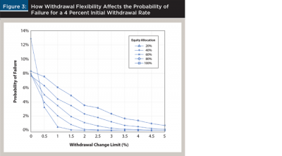
Figure 4 complements Figure 2. The two panels depict the relation between the expected growth rate of withdrawals and the choice of withdrawal flexibility. In Figure 4A, “average” growth is defined as the median real withdrawal growth rate. For inflexible withdrawal strategies, real growth was constrained to be zero unless the portfolio ran out of money. As the withdrawal change limit was relaxed, median withdrawal growth could diverge from zero. Whether withdrawals increased or decreased over time, on average, depended on the relation between the expected return of the portfolio (determined by the equity allocation chosen) and the initial withdrawal rate.
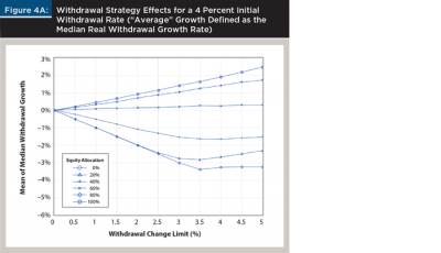
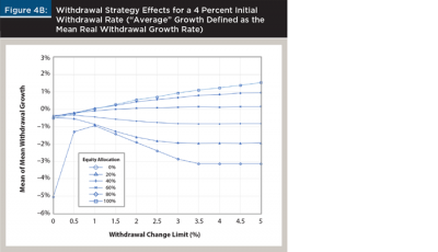
If the initial withdrawal rate is high relative to the portfolio’s expected return, we should expect to see real withdrawals adjust downward over time, and vice versa. The growth rates will be determined by the withdrawal change limits. Figure 4A shows a nearly linear relation between median real withdrawal growth rates and real withdrawal change limits. In Figure 4B, “average” is the mean real withdrawal growth rate. Mean withdrawal growth rates were more influenced by the large and uncontrollable withdrawal changes that occurred when a portfolio ran out of money. For example, 100 percent of trials ended in failure for an all-cash portfolio with an inflexible strategy that initially withdrew 4 percent. The median real withdrawal growth rate for each of those trials was 0 percent, because the withdrawal changes associated with running out of money were outliers. However, the mean growth rates, which included the effect of the outlier, were all negative. This is clear when comparing the two panels of Figure 4.
Households in retirement are subject to numerous risks. This paper was concerned with two of them: (1) uncertainty about lifestyle goals (associated with the level and volatility of future real withdrawals); and (2) uncertainty about legacy goals (associated with the level and volatility of terminal wealth).
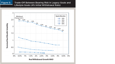
The third lever, real withdrawal change limits, effectively transfers some of the portfolio’s market risk from legacy goals to lifestyle goals. When the withdrawal strategy is inflexible, most of the market risk is expressed in terminal wealth volatility. Market risk only spills over into withdrawals when a portfolio “runs out of money.” When a household adopts a more flexible withdrawal strategy, some of the market risk is expressed in real withdrawal volatility, and the volatility of terminal real wealth is reduced.
This risk transfer from legacy goals to lifestyle goals is illustrated in Figure 5. The graph depicts the trade-off between bearing risk in legacy goals (measured on the y axis by terminal real wealth volatility) and bearing risk in lifestyle goals (measured on the x axis by mean of real withdrawal MAD). Figure 5 illustrates the results for a 4 percent initial withdrawal rate. The all-cash and all-equity portfolios are omitted for clarity. The trade-off is: as the real withdrawal change limit increased, terminal real wealth volatility decreased and the volatility of withdrawals increased. For a retired household, this corresponds to choosing to accept possible modest declines in lifestyle in order to improve the probability of achieving legacy goals.
Retirement Outcomes Under an Actuarial Spending Rule
Previous papers have advocated actuarial spending rules to mitigate longevity and sequence risk (Frank, Mitchell, and Blanchett 2011, 2012a, 2012b). Recall that constant fraction spending rules apply the same withdrawal rate to portfolio values, year after year. Actuarial spending rules based on annuity factors adjust the withdrawal rate upward with age to account for decreasing expected remaining life spans. Thus, actuarial spending rules excel at “spending down” wealth to a desired terminal value (perhaps zero).
Actuarial spending rules are closely related to constant fraction spending rules in one very important respect: withdrawals are very responsive to changes in portfolio value. However, those withdrawals may be too volatile for retired households with fixed expenses or low tolerance for changes in consumption. The purpose of this section is to investigate how combining an actuarial spending rule with withdrawal limits affects retirement outcomes.
For this part of the analysis, withdrawal flexibility choices were combined with a simple, but ubiquitous, actuarial spending rule: the required minimum distribution (RMD). Under the RMD, the withdrawal rate is the inverse of the life expectancy factor from the IRS Uniform Lifetime Table. It begins at 1/27.4 = 3.65 percent for age 70 and ends at 1/11.4 = 8.77 percent for ages 90 and above. In terms of the simulations, the constant rate used to determine spending was replaced by the increasing rates mandated by the RMD rule. The mechanism for applying real withdrawal change limits was unchanged. However, the interpretation of results changed in a subtle way.
In the literature on sustainable retirement income, the focus is on mitigating the probability of “running out of money.” Because the RMD rule represents a flexible withdrawal strategy, the probability of “running out of money” is negligible. In this analysis, the purpose of imposing withdrawal change limits on the RMD-mandated withdrawals was to make consumption smoother over time. Recall that the IRS requires that households withdraw a minimum amount from their tax-deferred accounts; it doesn’t require that they spend their entire withdrawal, or that they can’t withdraw more than the required minimum distribution. Retirees may be willing to trade an increased probability of failure for smoother consumption.
For this section, two minor changes were made to the experimental design. The household’s choice of initial withdrawal rate was replaced by the RMD withdrawal rate mandated for a 70-year-old (3.65 percent). Thereafter, the withdrawal rate increased annually as prescribed by the RMD rule. For clarity, only three withdrawal flexibility levels were considered: a 2 percent limit, a 5 percent limit, and no limit (unconstrained). Choosing no limit essentially implemented the RMD spending rule. The equity allocation choices remained the same: 0 percent, 20 percent, 40 percent, 60 percent, 80 percent, and 100 percent. As a result, the experiment in this section considered 18 permutations of two choices.
Figure 6A illustrates how a household’s choices affected expected levels of retirement income and terminal wealth. It plots median terminal real wealth versus the median sum of real withdrawals for the 18 choice permutations. Increasing a portfolio’s equity allocation increased the expected levels of both retirement outcomes under the RMD spending rule.
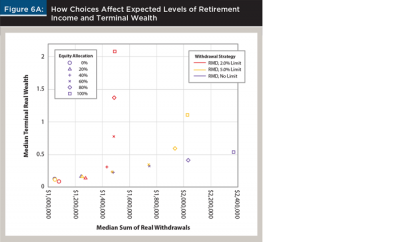
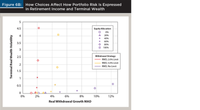
Figure 6 also shows results when comparing outcomes for a given equity allocation. For low equity allocations (40 percent and below), differences in withdrawal flexibility level had negligible effect on retirement outcomes. The differences became more pronounced for higher equity allocations. The unconstrained RMD withdrawal strategy worked as intended; it effectively “spent down” the household’s retirement assets. Increasing the equity allocation substantially increased the median sum of real withdrawals and only modestly increased median terminal wealth. In other words, the portfolio’s higher expected returns were expressed as higher retirement income, not higher terminal wealth.
Implementing a 2 percent real withdrawal change limit changed the picture. With relatively strict limits on withdrawal flexibility, the higher expected returns for portfolios with more than 40 percent equity resulted in higher median terminal real wealth, not higher median retirement income. The 2 percent limit on increases in real withdrawals inhibited the RMD rule’s ability to “spend down” wealth. When the withdrawal change limit was increased from 2 percent to 5 percent, the portfolio generated more income and terminal wealth was reduced, on average.
Figure 6B illustrates how a household’s choices affect how portfolio risk is expressed in retirement income and terminal wealth. The level of portfolio risk is, of course, determined by the choice of equity allocation. How that risk is borne by a household is determined by the choice of withdrawal flexibility. Figure 6B plots terminal real wealth volatility versus real withdrawal growth MAD. For every equity allocation, the unconstrained RMD spending rule resulted in the highest level of uncertainty about growth in real withdrawals. These high levels of uncertainty around retirement income are likely to be unsettling for retired households with fixed expenses or strong preferences for smooth consumption. Implementing limits on real withdrawal changes worked as intended; uncertainty around retirement income (as measured on the x axis by real withdrawal growth MAD) was effectively capped at the desired level (2 percent or 5 percent). When real withdrawal change limits were imposed, a fraction of portfolio risk was effectively shifted from being borne in consumption to being borne in terminal wealth.
Implications for Financial Planners
This paper demonstrated how moving the three choice levers (asset allocation, initial withdrawal rate, and withdrawal flexibility) affected the joint distribution of retirement outcomes in terms of future consumption and terminal wealth. Retiree preferences for these outcomes are highly idiosyncratic; they depend on the household’s goals, preferences, and circumstances. Therefore, it is important for financial planners to understand how and why moving the levers affects the trade-offs faced by retirees.
The withdrawal rate lever is the primary means by which retirees alter the trade-off between consumption and legacy goals. Increasing static withdrawal rates essentially shifted the whole distribution of terminal wealth outcomes toward zero. Perhaps as expected, high static withdrawal rates were associated with lower expected terminal wealth and lower probability of success.
The asset allocation lever determines the amount of market risk to be borne by the household. Under an inflexible withdrawal strategy, a higher equity allocation increased both the mean and the dispersion of terminal wealth. These have opposite effects on the probability of depleting wealth. As a result, the asset allocation lever had little overall impact on a retired household’s “probability of success.” The result was different for legacy goals. Because legacy beneficiaries effectively possess a long call option on terminal wealth, a higher equity allocation made their claim more valuable.
The withdrawal flexibility lever serves a key role in affecting retirement outcomes. It is well-known that reducing withdrawals after a market downturn reduces the risk of running out of money. This analysis showed that even modest withdrawal flexibility (under 2 percent) could have a significant effect. Withdrawal flexibility effectively transferred some market risk from a household’s terminal wealth to its consumption. The appropriate level of withdrawal flexibility should account for the household’s competing goals and preferences for consumption smoothness. If a retired household prefers lifestyle over legacy goals, it may be appropriate to increase withdrawal rates over time, as suggested by some actuarial withdrawal strategies. Actuarial withdrawal strategies excel at “spending down” wealth.
Eliciting a household’s preferences for “smoothness” may be a worthwhile exercise. The conversation should be framed in relevant terms. In other words, what would withdrawal flexibility mean in the event of a market downturn? Assume the client is a newly retired household with $1 million in assets, and that they have decided to withdrawal $40,000 in the first year to support their lifestyle. A market downturn would require a reduction in next year’s budget. What discretionary spending would they be willing to do without? A 2 percent withdrawal change limit would correspond to budget cut of about $67 per month. That might mean forgoing dinner out once per month. Households may be willing to make such a sacrifice to increase their probability of success.
Because retiree goals in terms of lifestyle and legacy can be easily related to income and terminal wealth, a case can be made for featuring regular Monte Carlo simulation in the retiree planning and decision-making process. Households exhibit unique preferences with respect to risk aversion and consumption smoothness, so no “universal” spending rule can be fully satisfactory. Monte Carlo simulation, including modeling of the three choice levers and realistic representation of retirement outcomes (in terms of both lifestyle and legacy goals), can be critical to investor success.
Endnotes
- See the “2016 Mid-Year AICPA CPA Personal Financial Planning Trends Survey” available at aicpa.org/InterestAreas/PersonalFinancial Planning/Community/DownloadableDocuments/PFP-Trends-Survey-MidYr.pdf.
- This statement implicitly assumes that the underlying portfolio has zero probability of a –100 percent return.
- Consider a household whose asset allocation/withdrawal strategy has a 10 percent probability of failure. A year later, their probability of failure would certainly be lower following a +20 percent portfolio return than following a –20 percent portfolio return.
References
Bengen, William P. 1994. “Determining Withdrawal Rates Using Historical Data.” Journal of Financial Planning 7 (4): 171–180.
Bengen, William P. 1996. “Asset Allocation for a Lifetime.” Journal of Financial Planning 9 (4): 58–67.
Bengen, William P. 2001. “Conserving Client Portfolios During Retirement, Part IV.” Journal of Financial Planning 14 (5): 110–119.
Blanchett, David M. 2017. “The Impact of Guaranteed Income and Dynamic Withdrawals on Safe Initial Withdrawal Rates.” Journal of Financial Planning 30 (4): 42–52.
Cooley, Phillip L., Carl M. Hubbard, and Daniel T. Walz. 1998. “Retirement Savings: Choosing a Withdrawal Rate that Is Sustainable.” AAII Journal 20 (2): 16–21.
Epstein, Lawrence, and Stanley Zin. 1989. “Substitution, Risk Aversion, and the Temporal Behavior of Consumption and Asset Returns: A Theoretical Framework.” Econometrica 57 (4): 937–969.
Epstein, Lawrence, and Stanley Zin. 1991. “Substitution, Risk Aversion, and the Temporal Behavior of Consumption and Asset Returns: An Empirical Investigation.” Journal of Political Economy 99: 263–286.
Fama, Eugene F., and Kenneth R. French. 2002. “The Equity Premium.” Journal of Finance 57: 637–659.
Frank, Larry R., John B. Mitchell, and David M. Blanchett. 2011. “Probability-of-Failure-Based Decision Rules to Manage Sequence Risk in Retirement.” Journal of Financial Planning 24 (11): 44–53.
Frank, Larry R., John B. Mitchell, and David M. Blanchett. 2012a. “An Age-Based, Three-Dimensional Distribution Model Incorporating Sequence and Longevity Risks.” Journal of Financial Planning 25 (3): 52–60.
Frank, Larry R., John B. Mitchell, and David M. Blanchett. 2012b. “Transition Through Old Age in a Dynamic Retirement Distribution Model.” Journal of Financial Planning 25 (12): 42–50.
Guyton, Jonathan T., and William J. Klinger. 2006. “Decision Rules and Maximum Initial Withdrawal Rates.” Journal of Financial Planning 19 (3): 49–57.
Jaconetti, Colleen M., Francis M. Kinniry, and Michael A. DiJoseph. 2013. “A More Dynamic Approach to Spending for Investors in Retirement.” Vanguard Research Paper available at pressroom.vanguard.com/nonindexed/2013.10.23_A_more_dynamic_approach_to_spending.pdf.
Pfau, Wade D. 2015. “Making Sense Out of Variable Strategies for Retirees.” Journal of Financial Planning 28 (10). 42–51.
Pfau, Wade D. 2017. How Much Can I Spend in Retirement? A Guide to Investment-Based Retirement Income Strategies. McLean Va.: McLean Asset Management Corp.
Zolt, David. 2013. “Achieving a Higher Safe Withdrawal Rate with the Target Percentage Adjustment.” Journal of Financial Planning 26 (1): 51–59.
Citation
Scruggs, John T. 2019. “Asset Allocation and Withdrawal Strategies: Three Levers for Managing Retirement Outcomes.” Journal of Financial Planning 32 (6): 39–49.