Journal of Financial Planning: July 2011
Manoj Athavale, Ph.D., is an associate professor in the department of finance and insurance at the Miller College of Business at Ball State University in Muncie, Indiana.
Joseph M. Goebel, Ph.D., is an assistant professor, also in the department of finance and insurance at the Miller College of Business at Ball State University.
Executive Summary
- A common conundrum faced by most people approaching retirement is the amount of money they can safely withdraw from their retirement portfolio without the risk of depleting the portfolio over their retirement horizon. The advice that most retirees will hear is the 4 percent rule—a retiree who faces normal retirement conditions can make an annual inflation-adjusted withdrawal equal to 4 percent of the original portfolio without risk of depleting the portfolio.
- This rule of thumb has helped bring a disciplined approach to retirement withdrawal strategy. However, tests of the 4 percent rule using simulation methodology have assumed that expected returns are drawn from a lognormal distribution—an assumption that lacks empirical support.
- The important question, therefore, is whether the choice of method used to represent the future affects estimates of the sustainability of a retirement portfolio.
- We test the 4 percent rule by creating plausible retirement scenarios using standard methodology, but assuming that expected returns can conform to various distributions.
- Our analysis indicates that a 4 percent withdrawal rate will result in portfolio failure with greater probability (18 percent) than previously believed, and the truly “safe” withdrawal rate—2.52 percent—is significantly smaller than previously believed.
Retirement planning is an important part of the financial planning process, and financial planners are often called to assist their clients in formulating retirement plans. Two common but related questions most retirees face are: (1) how much money do I need to have accumulated prior to retirement, and (2) how much consumption expenditure will my retirement portfolio sustain over the retirement horizon? Answers to such questions are increasingly relevant to financial planners as baby boomers approach retirement. Many of the individuals approaching retirement may not have accumulated a retirement portfolio that will sustain consumption at current levels—life expectancy has been increasing, and the proportion of retirees covered by a defined benefit plan is decreasing. Further, the recent turmoil in the financial markets has adversely affected retirement portfolio balances and may have affected retirees’ appetite for the risk inherent in equity-type investments.
In the process of trying to ensure a financially secure retirement, individuals go through two distinct phases: an accumulation phase and then a draw-down phase during which periodic withdrawals are made from the accumulated portfolio. A concern for many retirees is the ability of their portfolio to sustain their retirement consumption; that is, retirees would need to know the amount that can be safely withdrawn from the portfolio every year without the risk of depleting the portfolio during their lifetimes. The “4 percent rule” is a generally accepted rule of thumb that assists in estimating the amount that can be safely withdrawn from a retirement portfolio. In its most general form, the rule suggests that a retiree with a reasonably diversified retirement portfolio may make inflation-adjusted annual withdrawals equal to 4 percent of the initial portfolio balance. Bengen (1994) reached this conclusion based on his observation that a 4 percent inflation-adjusted annual withdrawal had never caused a portfolio to be exhausted in any prior 33-year retirement period. The primary advantage of the 4 percent rule is the simplicity with which this rule can be explained to retirees and the ease with which the rule can be implemented. The 4 percent rule brings a simple, disciplined approach to retirement consumption and to the management of the retirement portfolio, and tries to balance the two sides of the withdrawal rate dilemma: withdraw too much and face the negative consequences of outliving the retirement portfolio or withdraw too little and under-live the retirement potential.
Numerous studies have analyzed and built on the 4 percent rule by refining portfolio investment strategies, fine-tuning withdrawal strategies, and improving on data and analytical methods. Some of these studies have concluded that the 4 percent withdrawal rate can be achieved, but is accompanied by some risk of premature portfolio exhaustion, and other studies have suggested that the 4 percent withdrawal rate is too conservative and inefficient and that higher withdrawal rates are feasible. In interviews with seasoned financial planners, Stolz (2009) found a similar bipolarity in assessing retirement portfolio liquidation strategies, and expressed a sense that today’s financial environment just might require a new approach to analyzing sustainable distribution rates. The current retirement environment differs from that of the past, and changing circumstances may require a reconsideration of the conclusions and the assumptions that underlie the conclusions. Stolz did find that financial planners thought the 4 percent withdrawal rule was a good starting point for client-centric decisions about the retirement experience. However, Stolz noted that although simulation analysis was commonly used in estimating sustainable withdrawal rates, some financial planners were concerned that there was little justification for the commonly used assumption that returns were normally distributed.
Development of the 4 Percent Rule
The determination of a sustainable withdrawal rate has been addressed in a number of prior studies. Bierwirth (1994) conducted an ex-post analysis of 42 overlapping retirement experiences (the first corresponds to the 26-year retirement horizon of a person who retired in 1926, the second corresponds to the 26-year retirement horizon of a person who retired in 1927, etc.) for a person who wanted to maintain the nominal value of a diversified retirement portfolio over a 26-year retirement period. Bierwirth’s analysis showed that differences in investment return and inflation among the 42 retirement experiences would result in annual real consumption of 5.6 percent for the 1926 retiree, but only 3.3 percent for a 1937 retiree, with an average of 4.38 percent across all retirement experiences.
Bierwirth recognized the impact of the retiree’s investment decision on the value of the portfolio and consumption and demonstrated that the average annual real consumption would be 3.2 percent with a conservative portfolio and 5.4 percent with an aggressive portfolio. Although the conservative portfolio provided less income volatility, the aggressive portfolio could sustain greater consumption, leading Bierwirth to conclude that the aggressive portfolio (containing a greater proportion of equity) could be recommended as superior, assuming the retiree had the attributes of discipline and risk tolerance. Bierwirth also recognized the relevance of the timing of returns, not just the level of returns, in influencing the 42 retirement experiences. Bierwirth explained the apparent anomaly of lower real consumption in the 1940–1965 retirement period (as compared with 1954–1979) despite higher real returns as being caused by lower returns early in the retirement period and higher returns later in the retirement period, when they had less of an effect on the retirement experience.
Bengen (1994) recognized that average returns and average inflation are not a sound basis for computing the amount that could be withdrawn from a retirement portfolio, and that the long-term effects of certain financial catastrophes (for example, 1929–1931, 1937–1941, and 1973–1974) could overwhelm the averages. Bengen calculated portfolio longevity (number of years a retirement portfolio could sustain consistent consumption) using historical and extrapolated returns on a balanced portfolio to show that the retirement portfolios of people who retired during the 1926–1976 period and withdrew 4 percent of the initial balance every year adjusted for inflation would last at least 33 years, and in most cases would last 50 years or longer. Bengen’s research also suggested that stock allocations less than 50 percent reduced portfolio longevity and accumulated wealth, stock allocations as high as 75 percent may be appropriate depending on risk tolerance, and stock allocations greater than 75 percent reduced portfolio longevity, especially during financial downturns.
Testing the 4 Percent Rule
Over the past few years there have been numerous efforts to test the 4 percent rule and to improve its application. Pye (2000) used simulation methodology on a portfolio comprising varying proportions of equity (average annual return of 8 percent distributed lognormal), Treasury Inflation-Protected Securities or TIPS (average annual return of 3.7 percent), and cash (average annual return of 2 percent) to conclude that a 4 percent withdrawal rate was sustainable, but that portfolio sustainability was predicated on an assumption about average returns, and this assumption made an appreciable difference on the retirement experience and the terminal value of the portfolio. Similar results were obtained by Spitzer, Strieter, and Singh (2007), who used a large number of bootstrap simulations to conclude that a balanced portfolio could sustain a 4 percent withdrawal rate over a 30-year horizon, but was associated with a 6 percent chance of portfolio failure.
Two analytical techniques have been used to examine the possibility that a retiree may outlive the accumulated retirement portfolio: overlapping period models and simulation models. Overlapping period models apply the actual historical security return and inflation rates to current retirees, under the assumption that future market behavior will resemble the past, to determine the impact of those conditions on periodic portfolio returns and portfolio balances. Simulation models use past history to calculate the mean, standard deviation, and correlation for portfolio return and inflation. These values are then used to draw random values from a normal or lognormal distribution, and these randomly generated values are used in making inferences about expected periodic portfolio returns and portfolio balances.
An important question therefore is whether the choice of method used to represent the future affects estimates of the sustainability of a retirement portfolio. Cooley, Hubbard, and Walz (2003) used both methods to calculate portfolio success rates (the percentage of retirement experiences during which the retirement portfolio provided planned withdrawals and finished the period with a positive value) for a range of withdrawal rates, portfolio compositions, and payout periods. Their results showed that both models were generally consistent; a 4 percent withdrawal rate could be sustainable over a 30-year period with a balanced portfolio, but to ensure a 90 percent success rate, a larger allocation to equity and withdrawal rates of less than 4 percent were necessary.
The overlapping period methodology uses actual historical data and is easy to understand, but sample size is restricted to the available historical data. Further, the returns from the middle period are included in more overlapping periods than returns that occur at the beginning and end of the data period, and thus have a disproportionate impact on the results. Simulation methodology can generate large amounts of data for analysis, but various assumptions have to be made about the mean, standard deviation, and nature of distribution from which the sample will be drawn.
Many retirees have had anything but the perfect retirement experience; hence, Guyton (2004) analyzed the sustainable withdrawal rate for a single 1973 retirement scenario that provides a “perfect storm” planning exercise—incorporating an early period of high and prolonged inflation and two bear markets. Guyton adopted two significant innovations in his analysis. The first was the use of a many-asset-class portfolio that allowed for greater equity allocation than otherwise; the second was the use of various decision rules to determine target portfolio allocations and the sequence in which the asset-class balances were used to fund withdrawals, limitations on withdrawals when the portfolio underperformed, and limitations on inflation adjustments to the annual withdrawal. An important contribution of Guyton’s analysis was recognition that the upshot for the various decision rules applied during the course of retirement was a higher initial withdrawal rate (5.8 percent). The unresolved questions, however, were whether retirees would have the discipline to follow the three decision rules, the flexibility to reduce real consumption, and whether this single retirement scenario could apply to retirees in other periods.
Portfolio sustainability is fundamentally a function of three variables: asset allocation, life expectancy, and spending rates. These variables are not deterministic, and hence Milevsky and Robinson (2005) resorted to stochastic calculus to derive a closed-form expression for the probability the retirement portfolio would be depleted. This model assumed that a person begins retirement at age 65 with a balanced portfolio (5 percent real returns, 12 percent standard deviation, and returns are distributed lognormal), and remaining life expectancy at retirement would be exponentially distributed. The typical retiree, who consumes an inflation-adjusted amount equal to 4 percent of the initial portfolio every year, would face a 9 percent probability of portfolio ruin—a level that would be unacceptable to most retirees. The Milevsky and Robinson model could also be inverted to calculate the sustainable withdrawal rate—3.24 percent for a retiree willing to accept a 5 percent probability of ruin. Sustainable withdrawal rates estimated by the Milevsky and Robinson analytical model are lower than those estimated in prior studies that used overlapping period or simulation models.
Financing a constant 4 percent consumption plan using the volatile returns from a traditional retirement portfolio is fundamentally flawed. Generally, a constant consumption plan is best supported by a portfolio that generates corresponding constant returns. Scott, Sharpe, and Watson (2009) used simulation models to determine that 4 percent withdrawals from a portfolio that generated 6 percent real annual returns with 12 percent standard deviation over a 30-year horizon would have a 5.7 percent chance of portfolio failure. Scott, Sharpe, and Watson also observed that the 4 percent withdrawal rate imposed an opportunity cost and was therefore inefficient, and suggested that a strategy that included buying and selling 30-year European call options would enable the retiree to obtain the 4 percent rule’s distributions, but at lower cost. However, many practical issues should be addressed before their suggestions for analyzing retirement income preferences with utility functions and using dynamic reallocation and call-option strategies to maximize expected utility can be incorporated in retirement planning.
The Distribution of Returns
An important variable in the determination of the sustainable withdrawal rate is expectations of future returns. Theoretically, a $1 million portfolio invested to provide a risk-free real return of 2 percent can sustain real consumption of approximately $40,000 over a 35-year period with no residual estate, and such an outcome may currently be possible with long-term TIPS or inflation-indexed annuities. However, many of the available investment choices are not completely risk free; retirees may desire the greater expected returns from equity markets and may have a secondary investment objective of creating an estate for their heirs.
Equity portfolio returns are expected to be higher than bond portfolio returns but with greater variability. Simulations have commonly been used to project future conditions and provide retirees possible retirement scenarios. Simulation models can generate a substantial number of scenarios based on input parameters that can be conveniently changed based on borrower characteristics. Simulation analysis should generally produce robust results, but the quality of the analysis depends on underlying assumptions and inputs. Simulation analysis may provide biased results if expected returns are generated from unstable distributions or different distributions over time (Cooley, Hubbard, and Walz 2003). Analytical methods that place ill-advised reliance on a particular parametric return distribution and on historical data as an indicator of the future may suffer serious mismeasurement of risk (Gosling 2010). Specifically, because the random returns used in simulation analysis are drawn from an assumed distribution, the results of the simulation may be biased if future returns do not conform to that distribution, and biased results may lead to misleading inferences.
A common assumption in previous studies is that returns are generated from a lognormal distribution. (Note that the normal and lognormal distributions are closely related; a lognormal distribution is the probability distribution of a random variable whose logarithm is normally distributed). However, the distribution of stock returns is known to be non-normal and heteroskedastic1 (Nelson and Kim 1993). The empirical distribution of returns has been observed to have more distributions around the mean and fatter tails than the normal distribution, and skewed distributions offer more flexibility in modeling returns by removing the constraint of symmetry in returns. Harvey and Siddique (2000) and Dittmar (2002) found that higher-order moments are relevant in explaining equity returns. Levy and Duchin (2004) therefore conducted a study to determine which theoretical distribution best fits the observed distribution of returns for various asset classes and holding periods, and found that the logistic distribution was generally the best fit, though in a few instances other distributions could also describe the observed returns.
Data and Analysis
Expected portfolio returns cannot be known with certainty; hence, standard methodology draws random returns for the desired retirement horizon from a theoretical distribution. Further, portfolio returns depend on asset allocation, which varies based on risk tolerance. We therefore restrict our analysis to a retiree who has accumulated a retirement portfolio positioned to provide an annual real return of 5.1 percent with a standard deviation of 12 percent. These parameters are consistent with Bengen’s 5.1 percent return with a 60/40 portfolio (1994), Milevsky and Robinson’s 5 percent return and 12 percent standard deviation with a 50/50 portfolio (2005), and Scott, Sharpe, and Watson’s 6 percent return and 12 percent standard deviation with a 60/40 portfolio (2009).
We began our analysis by drawing random annual returns for 35 periods from a distribution that had a mean of 5.1 percent and a standard deviation of 12 percent. These 35 returns correspond to the annual returns a retiree is likely to experience over a 35-year retirement horizon. We relax the assumption that portfolio rates of return follow any single distribution, and conduct the process for 10 continuous probability distributions (Beta, Extreme, Gamma, Laplace, Logistic, Lognormal, Pert, Rayleigh, Wakeby, and Weibull), most of which are characterized by multiple parameters to represent the location, scale, and shape of the distribution. These parameters can be adjusted to ensure the desired mean, standard deviation, and bounds. The process was then repeated so that we have 10 scenarios for each of the 10 distributions, for a total of 100 retirement scenarios. The simple average annual real return across the 100 scenarios was 4.93 percent with standard deviation of 11.6 percent. Some of these retirement scenarios are presented in Table 1.
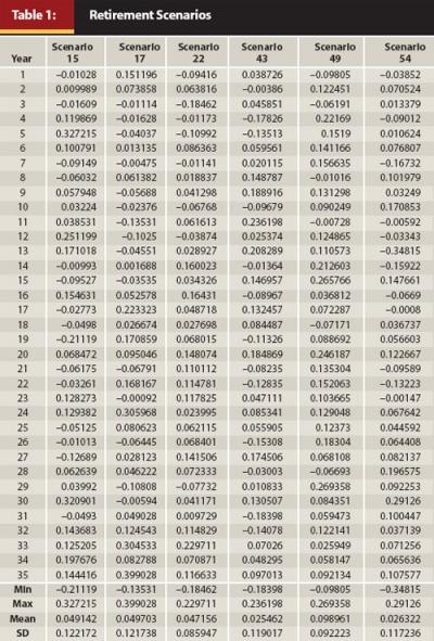
The six scenarios presented in Table 1 represent possible annual real returns over a 35-year retirement horizon. The range of returns and the mean and standard deviation appear plausible. Note that the 35-year retirement horizon was selected because Bengen (1994) found that in no case had a 4 percent withdrawal rate caused a portfolio to be exhausted before 33 years. Second, based on current estimates for a couple retiring at age 65, there is a 25 percent chance that one of them will live to age 97. We assume that returns accrue to a $1 million portfolio at the end of each year and withdrawals are made at the end of each year. We determined portfolio outcome (success or failure) by creating a 35-year retirement “ledger” showing returns, withdrawals, and balances for each year. The process was repeated for each of the 100 scenarios. One such retirement experience is presented in Table 2.
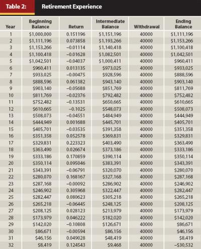
Table 2 presents the 35-year retirement experience of a retiree whose portfolio obtains the Scenario 17 returns (average return is 4.97 percent, standard deviation is 12.17 percent, minimum return is –13.53 percent, and maximum return is 39.90 percent) presented in Table 1. Unfortunately for our retiree, the entire portfolio was exhausted after 31 years. The risk inherent in a portfolio that includes equity causes portfolio returns to fluctuate from year to year; thus, in some periods the withdrawal exceeds returns, drawing down on the balance, and the reduced balance may not be large enough to benefit from higher returns in subsequent periods. Portfolio exhaustion may be exacerbated by negative runs. A sequence of negative returns early during retirement may cause the portfolio balance to fall, and the reduced balance may not be able to benefit from subsequent higher earnings.
Table 2 clearly highlights the risks associated with financing fixed consumption with variable returns. During 24 of the first 31 years, the portfolio returns were insufficient to finance the 4 percent withdrawal rate, leading to portfolio failure after 31 years. A substantially exhausted portfolio cannot benefit from superlative returns in subsequent years; high returns in years 32 to 35 are futile to this retirement experience. Note that although a retirement portfolio is likely to experience both positive and negative returns, it would be better for good years to occur earlier in retirement.
We computed portfolio outcomes in a similar manner for each of the 100 scenarios. Although most scenarios resulted in portfolio success (the portfolio was able to sustain a 4 percent withdrawal rate over the 35-year period), we were surprised by the proportion of scenarios that resulted in portfolio failure—18 of the 100 scenarios. In order to be consistent with some of the other studies mentioned previously, we redefined portfolio success by shortening the retirement period to 30 years. The portfolio failure rate dropped to 14 percent, but is still higher than Milevsky and Robinson’s 9 percent (2005), Spitzer, Strieter, and Singh’s 6 percent (2007), and Scott, Sharpe, and Watson’s 5.7 percent (2009). We also computed the portfolio balance (in real dollars) at the end of the 35-year retirement period for successful scenarios. Finally, we inverted our model to calculate the sustainable withdrawal rate (the maximum rate at which a given portfolio may be drawn down without depleting the portfolio before the end of the 35-year retirement horizon) for each of the 100 scenarios. Portfolio outcomes for the six previously described retirement scenarios are presented in Table 3.
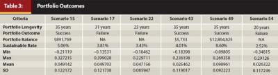
Table 3 illustrates portfolio outcomes for 6 of the 100 retirement scenarios. In Scenarios 15, 43, and 49 the portfolio was able to sustain a 4 percent withdrawal rate over a 35-year retirement horizon, while Scenarios 17, 22, and 54 ended with portfolio failure. We would like to make a few observations about the portfolio outcomes illustrated by these six scenarios. First, scenarios in which average returns exceed the withdrawal rate do not necessarily lead to portfolio success (Scenario 17 resulted in portfolio failure while Scenario 15 succeeded). Second, scenarios in which average returns are lower than the withdrawal rate do not necessarily result in portfolio failure (Scenario 43 resulted in portfolio success while Scenario 54 failed). Third, low standard deviations do not necessarily result in portfolio success (Scenario 22 ended in portfolio failure). Fourth, while some retirement experiences will result in failure, the nature of equity returns causes others to be immensely successful (scenario 49 with high returns and low standard deviation had amassed an estate worth more than $12 million). Taken together, these findings suggest that although larger returns and smaller standard deviations contribute to portfolio success, these are not sufficient conditions to ensure success, and other factors including the timing of returns and the occurrence of negative or positive runs may also be important.
Our analysis shows that the sustainable withdrawal rate for the 100 risky scenarios in our selection ranges from 2.52 percent to 10.59 percent with an average of 5.69 percent. The range of sustainable withdrawal rates indicates that a retiree could make a 2.52 percent annual withdrawal from a risky portfolio, and that such a withdrawal could sustain a 35-year retirement through almost any returns scenario. A retiree can, of course, choose from innumerable asset allocation and withdrawal strategy combinations, but based on our analysis, we would like to highlight the following:
- A 4 percent inflation-adjusted withdrawal from a retirement portfolio that yields a risk-free average annual real return of 2 percent will last 35 years with no portfolio balance at the end of that period.
- A 2.52 percent inflation-adjusted withdrawal from a retirement portfolio that yields an average annual real return of 5.1 percent with 12 percent standard deviation will last 35 years, but with no portfolio balance at the end of that period in some cases and substantial portfolio balances in others.
- A 4 percent inflation-adjusted withdrawal from a retirement portfolio that yields an average annual real return of 5.1 percent with 12 percent standard deviation will last 35 years with 82 percent probability. In the extreme, the portfolio might sustain consumption for only 20 years, or might last 35 years and accumulate a substantial estate.
People approaching retirement can be better prepared for the retirement decision if they are informed about the full range of retirement experiences possible, and the three points above can assist retirees in selecting asset allocation and withdrawal strategies based on their unique financial situations and risk tolerances.
Conclusion
A common question faced by most retirees is the amount that can be consistently withdrawn from a portfolio without depleting the portfolio before the end of the retirement period. The consistent advice most investors and retirees will hear is that a 4 percent withdrawal rate can be sustained throughout the retirement period. The efficacy of this rule has been tested in recent years, often using simulations to model for expected returns. However, Milevsky and Robinson have previously cautioned that simulation models such as those used in tests of the 4 percent rule are subject to misspecification because many return scenarios are not adequately captured in a lognormal distribution.
If tests of the 4 percent rule are dependent on an assumption about the distribution of expected returns, the results are likely to be incorrect if other distributions occur in the future. It is therefore necessary to examine the impact of the assumption on the outcomes. In this study, we have refined the 4 percent rule by relaxing the common assumption that expected returns can be described by a lognormal distribution.
Our results indicate that a 2.52 percent withdrawal rate could be sustained in each of our randomly generated scenarios, but a 4 percent withdrawal rate is associated with an 18 percent probability of portfolio failure. The proportion of portfolio failures associated with the 4 percent withdrawal rate (18 percent) is higher, and the sustainable withdrawal rate (2.52 percent) is lower, than previously reported. Further, adverse market conditions coupled with a 4 percent withdrawal rate can completely deplete the retirement portfolio in as few as 20 years.
Although some retirees may have lower risk tolerances and prefer relative certainty, others may desire higher current consumption but nevertheless hope for a successful retirement experience. Unfortunately, hope does not constitute good financial planning or retirement strategy. The role of the financial planner in this process, of course, is providing the client with objective guidance based on knowledge of the past and educated estimates of what the future may hold.
The 4 percent rule, like any rule of thumb, has its limitations when applied to specific circumstances. Many variables influence the retirement experience, and determining sustainable retirement consumption is at best an inexact science. There are, however, many ways a financial planner can remain engaged with a client to improve the probability that a client’s retirement will be successful. Most importantly, it may be necessary to emphasize the importance of certainty in sustaining retirement consumption. After all, a 2 percent risk-free real return can sustain an annual 4 percent inflation-adjusted withdrawal over the entire 35-year retirement. This can currently be achieved with financial instruments such as TIPS and annuities. A single-premium immediate annuity with an inflation rider can also assist the retiree to mitigate longevity risk, and there are many situations in which this option is optimal for retirees (Davidoff, Brown, and Diamond 2005).
Endnote
- Investopedia.com offers the following definition for heteroskedastic: Most financial instruments, such as stocks, follow a heteroskedastic error pattern. For example, in regression, a mathematical relationship between a stock and some other type of measure is to be discovered over a period of time; the error found between the line of best fit and the actual data point will vary—for instance, as each variable gets larger the error may increase.
References
Bengen, W. 1994. “Determining Withdrawal Rates Using Historical Data.” Journal of Financial Planning 7: 171–180.
Bierwirth, L. 1994. “Investing for Retirement: Using the Past to Model the Future.” Journal of Financial Planning 7: 14–24.
Cooley, P., C. Hubbard, and D. Walz. 2003. “A Comparative Analysis of Retirement Portfolio Success Rates: Simulation Versus Overlapping Periods.” Financial Services Review 12: 115–128.
Davidoff, T., J. Brown, and P. Diamond. 2005. “Annuities and Individual Welfare.” American Economic Review 95: 1573–1590.
Dittmar, R. 2002. “Nonlinear Pricing Kernels, Kurtosis Preference, and Evidence from the Cross Section of Equity Returns.” Journal of Finance 57: 369–403.
Gosling, S. 2010. “A Scenarios Approach to Asset Allocation.” Journal of Portfolio Management 37: 53–66.
Guyton, J. 2004. “Decision Rules and Portfolio Management for Retirees: Is the ‘Safe’ Initial Withdrawal Rate Too Safe?” Journal of Financial Planning 17: 54–62.
Harvey, C., and A. Siddique. 2000. “Conditional Skewness in Asset Pricing Tests.” Journal of Finance 55: 1263–1295.
Levy, H., and R. Duchin. 2004. “Asset Return Distributions and the Investment Horizon.” Journal of Portfolio Management 30: 47–62.
Milevsky, M., and C. Robinson. 2005. “A Sustainable Spending Rate Without Simulation.” Financial Analysts Journal 61: 89–100.
Nelson, C., and M. Kim. 1993. “Predictable Stock Returns: The Role of Small Sample Bias.” Journal of Finance 48: 641–661.
Pye, G. 2000. “Sustainable Investment Withdrawals.” Journal of Portfolio Management 26: 73–83.
Scott, J., W. Sharpe, and J. Watson. 2009. “The 4% Rule—At What Price?” Journal of Investment Management 7: 31–48.
Spitzer, J., J. Strieter, and S. Singh. 2007. “Guidelines for Withdrawal Rates and Portfolio Safety During Retirement.” Journal of Financial Planning 20: 52–59.
Stolz, R. 2009. “Withdrawal Rules of Thumb: Seductively Simple, yet with Limitations.” Journal of Financial Planning 22: 22–27.
This is what the current study does: First, we present a review of some of the important milestone studies that initiated the 4 percent debate and influenced the methodology used in testing the efficacy of the 4 percent rule. Second, we relax the assumption that portfolio rates of return follow any particular distribution and examine whether a reasonably diversified retirement portfolio would be able to sustain a 4 percent withdrawal rate over a 35-year retirement horizon. Finally, we make recommendations financial planners may adapt in retirement discussions with their clients.