Journal of Financial Planning; July 2011
David M. Blanchett, CFP®, CLU, AIFA®, QPA, CFA, is the director of consulting and investment research for the Retirement Plan Consulting Group at Unified Trust Company in Lexington, Kentucky.
Executive Summary
- The analysis conducted for this paper suggests that the probability of a retiree actually needing income from a guaranteed minimum withdrawal benefit (GMWB) annuity, versus the income that could be generated from a taxable portfolio with the same value, is approximately 3.4 percent for males, 5.4 percent for females, and 7.1 percent for a couple, given current prevailing lifetime distribution factors (or guaranteed withdrawal rates).
- However, the net “cost” of the GMWB annuity from the perspective of the annuitant as a percentage of annuity total value is approximately 6.5 percent, 6.1 percent, and 7.4 percent of the initial portfolio value for males, females, and couples, respectively (again, given current lifetime distribution factors for GMWB annuities).
- Because an annuity is a form of insurance, it would not be expected to have a positive average expected value, and will therefore compare unfavorably to non-annuity portfolios in “average” scenarios. The real question for a retiree is whether perceived benefits are greater than or equal to the cost of the insurance.
- Based on the results of this study, the guaranteed income protection in a GMWB annuity may be a relatively inexpensive form of “longevity insurance,” especially from a behavioral finance perspective, as retirees greatly fear outliving their retirement income. Although the current guaranteed rate environment is not generally favorable from an absolute average net value perspective, the author contends that GMWB-type features hold significant promise and are a viable strategy for managing longevity risk for a retiree.
Annuities that include guaranteed minimum withdrawal benefits (GMWBs) are becoming increasingly popular solutions for retirees seeking to minimize longevity risk. Unlike traditional annuities, or guaranteed lifetime income benefit (GLIB) annuities, which typically require the retiree to annuitize his or her entire account balance for a guaranteed lifetime income stream, annuities with GMWB riders guarantee lifetime income while allowing any remaining portfolio value to pass to the designated beneficiary at the death of the annuitant. This design alleviates a common fear among retirees about transferring total control of their retirement savings as well as the possibility they will die shortly after the annuitization date, thereby realizing only a portion of the total cost of the annuity.
In order for a retiree to benefit from a GMWB annuity rider, two things must happen: an alternative taxable equivalent portfolio must be no longer able to fund the expected withdrawal, and the annuitant must still be alive. The GMWB rider serves as “insurance” should these two events occur. Because an annuity is a form of insurance, we should not expect it to “pay off” on average. The true question is whether the cost of insurance provided by the annuity is equivalent to or greater than the perceived benefits to the annuitant. Attempts to quantify the true value of GMWB annuities have led to varied conclusions on this issue (notably, Chen 2007, and Huebscher 2011). The objective of this paper is to provide the reader information about the true “cost” of GMWB annuities. This analysis will help the reader more easily compare GMWB annuities to other longevity solutions and provide a framework to determine whether the potential benefits of GMWBs are worth the price.
Guaranteed Minimum Withdrawal Benefit Riders
GMWB annuity riders guarantee a minimum level of income for life and allow the annuitant to pass on his or her portfolio account balance to a beneficiary if there is any remaining policy value at the time of death. GMWB riders are also sometimes known as guaranteed lifetime withdrawal benefits (GLWBs). The guaranteed percentage, also known as the lifetime distribution factor, is based on the age of the annuitant at the time of the first withdrawal and typically increases the older the annuitant is at first withdrawal. The lifetime distribution factor is applied to what’s known as the “benefit base,” which is typically the greater of the current policy total dollar value or the maximum value at each of the previous policy anniversary dates. Some GMWB products have additional valuation methods, such as guaranteed crediting rates, that guarantee minimum increases in the benefit base through time.
The annuitant receives a fixed percentage of the benefit base—the lifetime distribution factor—based on the age of the retiree at the time of the first withdrawal. For example, if a male retiree age 65 invested $1 million in a GMWB annuity and received a lifetime distribution factor of 5 percent, he would be guaranteed income of at least $50,000 per year for life from the annuity. If the annuity portfolio value were to increase to $1.1 million on the second anniversary date, the benefit base would “step up” to $1.1 million and the guaranteed lifetime income amount would increase to $55,000. If the portfolio value were to fall to $900,000 the following year and were to never again exceed $1.1 million in value, the guaranteed withdrawal amount would still be based on the high-water mark value for the annuity, which was $1.1 million. Therefore, the annual income generated from the GMWB annuity would be $50,000 in year one, $55,000 in year two, and $55,000 per year thereafter until the annuitant dies. Alternatively, if the portfolio value increased to greater than $1.1 million at some point in the future, the guaranteed lifetime income would increase to 5 percent times that amount (in this example).
Lifetime distribution factors tend to increase for older annuitants. Xiong et al. (2010) note that 5.5 percent is a common lifetime distribution factor for those annuitants taking their first withdrawals at age 70, and 6 percent is common for those age 75. The actual lifetime distribution factor will vary by annuity provider, as will the ability to access the funds after annuitization. Surrender penalties and fees to access the annuity monies may apply based on the annuity provisions. At death, any remaining contract value in the GMWB annuity would be paid to a designated beneficiary. Even if the value of the GMWB annuity portfolio drops to $0 during the annuitant’s lifetime, the annuitant is still guaranteed lifetime income.
According to Xiong et al., the typical GMWB rider fee ranges from 60 to 90 basis points (bps). The fee will vary depending on the provisions of the GMWB rider, such as the available asset allocation range, the frequency of benefit base reset, etc. Usually the higher the fee, the more generous the lifetime distribution factor. Xiong et al. also provide useful information regarding the impact of GMWB rider provisions, such as portfolio volatility. Xiong et al. note that standard option pricing theory states that portfolios with higher volatility (standard deviation) have higher option prices. Because the GMWB rider is essentially a lifetime put option, if the fee associated with the GMWB rider doesn’t vary by equity allocation (which is common), investors are best served investing in the most aggressive portfolio possible inside the annuity. In response to this, though, many providers have maximum allowable equity allocations in GMWB policies (such as 70 percent).
GMWB Annuity Income
The actual income received from a GMWB annuity will vary depending on the annuity features and the lifetime distribution factor. The actual GMWB annuity dollar benefit amount is not directly tied to inflation, but rather the account’s benefit base. While the benefit base may increase with inflation (as markets increase), this may not necessarily occur, considering that withdrawals are going to be taken from the account annually, decreasing its value. The expected percentile cash flows from a 5 percent GMWB annuity for a male age 65 with a 60 percent equity allocation based on a 25,000-run Monte Carlo simulation are included in Figure 1. An inflation-adjusted initial withdrawal amount, growing at 3 percent annually, is also included in Figure 1 to give the reader a proxy for how well the nominal cash flows from the portfolio keep pace with inflation.
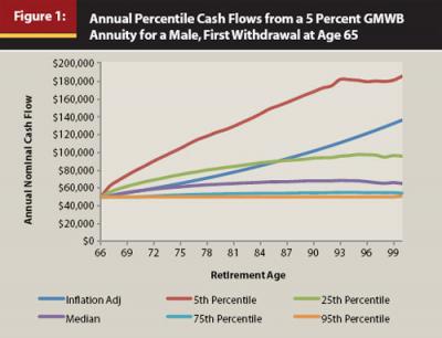
The median expected cash flow from the GMWB annuity in Figure 1 grows at a rate roughly equivalent to inflation for the first eight years, but then continues to increase at a decreasing rate. By the 15th year, the median cash flow is only increasing by roughly 1 percent per year. By the time the annuitant is 90 years old, or 25 years into retirement, the median expected GMWB annuity annual income is only approximately 68 percent of the inflation-adjusted value, at $68,000 and $100,000, respectively. Note, though, the median cash flow amount is greater than the initial cash flow amount of $50,000 for all retirement years. Even the 75th percentile cash flow (worst one run in four) is higher than the $50,000 initial cash flow for each year in retirement.
The GMWB Debate
Who knew annuity benefits could be so exciting? The varied findings of Chen (2007) and Huebscher (2011) suggest the debate regarding the potential benefit of GMWB riders is far from over. Chen conducts a robust analysis on the potential benefit of GMWB riders and finds that adding a variable annuity with a GMWB rider to a retirement portfolio results in lower total negative income returns, lower semi-standard deviation, higher average income returns, and higher total-income withdrawals. This is accomplished by replacing the fixed-income portion of a portfolio with an annuity with a GMWB rider, which is a reasonable assumption given the guaranteed nature of GMWB rider income and the actual investing decisions made by annuitants with lifetime income guarantees (Milevsky 2007).
Huebscher conducts a separate analysis using some of the same key assumptions as Chen and concludes that Chen’s study is “based on flawed methodology and has limited, if any, practical value.” Huebscher’s two primary critiques are that Chen only considered one scenario in his analysis, where the investor lives to age 90, and that Chen only considered sensitivity to his result of changes in the fee structure and in the equity/fixed-income allocation, not the expected return for the fixed-income component of the portfolio and the initial payout percentage for the annuity. Huebscher’s analysis dynamically incorporates mortality, and he finds little benefit from GMWB riders, noting that the GMWB rider is ultimately “handicapped by its fee structure.” In a counter to Huebscher’s analysis, Chen (2011) states that “Huebscher’s article is filled with material flaws.”
Similar to Huebscher’s study, the analysis conducted for this paper uses a more advanced mortality framework than Chen’s analysis, which is based on a single-scenario assumption. This author would contend that Chen’s single-scenario assumption was not impractical, though, given the number and type of varying simulations Chen conducted. However, this analysis assesses the benefit of GMWB annuities using a more advanced methodology than the approach taken by Huebscher or Chen and considers significantly more scenarios. The potential benefit of GMWB annuities for males, females, and couples is also addressed, while past research has primarily focused on their benefits to males.
Analysis
The objective of this paper is to provide the reader a framework to assess the true “cost” of GMWB annuities so they can more easily be compared to other longevity solutions. The analysis is conducted from the perspective of an annuitant, not the annuity provider, because an annuitant will have different preferences and discount rates applied to potential cash flows and benefits. For example, an individual retiree cannot pool longevity risk the way an insurance company can and therefore must purchase products (such as annuities) if he or she wishes to minimize or eliminate longevity risk.
There are two portfolios assumed for the analysis: one is an annuity that includes a GMWB rider and the second is a portfolio assumed to be invested in a taxable account. The assumed cash flows from the portfolio for each year of each run are identical. If the benefit base and subsequent cash flow increase inside the GMWB annuity, the same cash flow is assumed to be withdrawn from the taxable portfolio. This paper examines the relative benefit of purchasing a GMWB annuity versus “self-insuring” in a taxable account without a lifetime income guarantee.
The total cost of the GMWB annuity is assumed to be 200 bps for the male and female scenarios, and 220 bps for the couple scenario, based on a sampling of low-cost GMWB annuities—in particular the no-load annuity offered by Ameritas. The cost of the taxable portfolio is assumed to be 30 bps. The total GMWB annuity cost could be loosely viewed as the GMWB rider fee (about 80 bps for males and females and 100 bps for the couple), the annuity administration and M&E fees (about 60 bps), and the investment management fees in the annuity (about 60 bps). The investment expenses are relatively low, assuming the retiree invests primarily in a low-cost passive portfolio in either structure. A notable flaw in the methodology used to estimate the cost of the GMWB rider fee is that the rider fee is assumed constant regardless of the terms of the GMWB annuity. In reality, the cost of the GMWB rider will vary depending on its features (relative attractiveness).
An adviser fee (for example, 100 bps) is not included because it is assumed the adviser or financial planner would get paid whether investing the retiree monies in the passive portfolio or inside the GMWB annuity. A fee-only financial planner could just as easily sell a fee-only GMWB annuity and bill the client separately for his or her services, as could the financial planner receive a commission directly from the annuity sale. To truly understand the benefits of a GMWB annuity versus a taxable portfolio, any study must hold as many variables constant as possible. To assume the adviser must get paid 100 bps to sell the annuity but assume no fee comes from the taxable portfolio does not yield an equivalent comparison.
For simplicity purposes, taxes are ignored for the analysis. While it could be argued that ignoring taxes favors the GMWB annuities, given the less advantageous taxation of annuity income, that isn’t necessarily the case. The taxation of the portfolios would also be identical in a tax-deferred retirement account (such as a 401(k)). Taxation is therefore only an issue if the annuity is purchased with after-tax dollars.
Any growth in the annuity above investment will be taxed at ordinary income rates, unlike the taxable account, which will experience ordinary income rates and capital gains rates for securities held more than a year. Unlike the annuity, though, a taxable account will experience “tax return drag” every year, which reduces the compounded return of the portfolio during retirement. The fixed-income portion of the taxable portfolio would experience most (if not all) of its gains, reducing its compounded return. The equity piece would also experience some tax drag, either because of turnover in the portfolio or dividend income, depending on the tax efficiency of the portfolio.
Five different initial withdrawal ages are considered for this analysis: 60, 65, 70, 75, and 80. Life expectancy is based on the Social Security Administration 2006 Periodic Life Table (the most current life table available). The male and female for the couple scenarios are assumed to be the same age, and annual probabilities of survival are assumed to be independent. The couple is considered “alive” if either member is still living.
The Monte Carlo generator for this analysis was built in Microsoft Excel by the author. Conceptually, the analysis is conducted with a Monte Carlo portfolio generator that contains a Monte Carlo mortality generator overlay (or multiple mortality overlays when considering the couple scenario). The probability of being alive each year is randomly generated for each year of each run. This creates four possible scenarios for the taxable account each year:
- The retiree/couple is dead and the portfolio is still positive
- The retiree/couple is dead and the portfolio can no longer sustain the withdrawal
- The retiree/couple is alive and the portfolio is still positive
- The retiree/couple is alive and the portfolio can no longer sustain the withdrawal
A retiree/couple would only experience the relative “benefit” of the GMWB annuity if still alive when the taxable portfolio could no longer sustain the withdrawal. This is an important distinction, because it is only during these scenarios that the GMWB annuity actually “pays off.” Each scenario in the primary analysis is based on a 100,000-run Monte Carlo simulation, unless noted otherwise.
The GMWB benefit base is the maximum lifetime value of the portfolio for that run. The lifetime distribution factor is then applied to this value to determine the annual cash flow taken from the taxable portfolio and the GMWB portfolio. This analysis seeks to answer the question of whether it is worth self-insuring against the risks that can be hedged using a GMWB annuity. Any risk of the insurer defaulting was ignored.
All returns are based on a normal distribution. The equity allocation for the GMWB annuity was assumed to be 70 percent, while the equity allocation for the taxable portfolio was 50 percent. The equity allocation for the GMWB annuity was limited to 70 percent because most providers have maximum equity allocation provisions in their policies. Although the equity allocations in the portfolios were different, the same equity and bond returns were assumed for each scenario. This ensures the return environments are “equivalent” for the two tests when comparing cash flows. It would not be relevant to assume the 70 percent portfolio has a +30 percent return for a given year and the 50 percent equity portfolio has a return of –10 percent when comparing equivalent potential cash flows from the two portfolios. Basic market assumptions include: equity return of 10 percent (standard deviation 20 percent), bond return of 5 percent (standard deviation 7 percent), correlation of 0.2, and inflation at 3 percent.
Some readers may question the use of different equity allocations in the two portfolios. GMWB riders serve fundamentally as put options because they guarantee a fixed-income stream and are “bond-like” in nature. Given that the income is more certain from a GMWB annuity, its “actual” structural income risk allocation is more conservative than its actual portfolio equity allocation. Assuming a higher equity allocation in the GMWB annuity is also consistent with the behavior of actual annuity investors. Milevsky (2007) notes that the actual equity allocations for individual variable annuity contracts with lifetime income guarantees tend to be more aggressive than variable annuity contracts without income guarantees. Milevsky finds that annuitants age 65 and older with income guarantees have equity allocations approximately 20 percent higher than those without.
The GMWB Annuity Benefit
There are a variety of ways to assign a “value” to the GMWB annuity rider. One approach is simply to determine the probability the retiree/annuitant will actually ever need the rider versus the income that could be funded from the regular taxable portfolio. This information is included in Table 1, with the approximate range of current GMWB lifetime distribution factors highlighted in yellow for reference purposes.
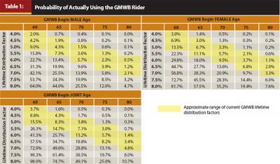
The probability of a retiree actually needing income from a GMWB annuity, versus the income that could be generated from a taxable portfolio with the same value, is approximately 3.4 percent for males, 5.4 percent for females, and 7.1 percent for a couple, given current prevailing lifetime distribution factors (or guaranteed withdrawal rates). These averages are based on the simple average of the likelihoods in the “approximate range of current GMWB lifetime distribution factors” illustrated in Table 1. The relative probability of needing the GMWB annuity coverage decreases with age given current lifetime distribution factors. A lifetime distribution factor of 5 percent is relatively common for 65-year-olds, yet the probability of a male, female, or couple actually needing the GMWB annuity, versus the income that could be funded from an outside portfolio, is 4.3 percent, 6.7 percent, and 8.3 percent, respectively. Just “needing” the income from the GMWB annuity, though, does not tell us the actual cash flows required from the GMWB annuity to fund retirement income. Needing the GMWB annuity to generate income for an average of 10 years is a very different benefit than requiring it to create income for a single year.
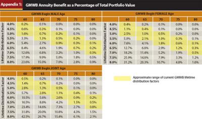
Figure 2 and Appendix 1 include information to help the reader understand the actual benefits an annuitant can expect to receive from a GMWB annuity. Figure 2 includes the expected total benefits received from 100,000 male “retirees” (Monte Carlo simulations) age 65 with $1 million invested in a GMWB annuity with a 5 percent lifetime distribution factor. The lifetime cash flows create an approximate normal distribution in Figure 2, with the largest annual need of $66 million dollars occurring when the “retirees” are 91 years old, or 26 years into retirement. The cash flows in Figure 2 are broken down into two sources: the initial lifetime distribution factor income and additional income above the rider that resulted from increases in the benefit base. These are listed separately because different discount rates are applied to the respective cash flows to determine the GMWB annuity benefit.
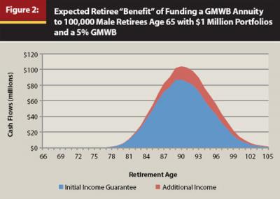
By taking the net present value of the annual cash flows, it is possible to determine the total benefit expected by the GMWB annuitants. The discount rate for the initial guaranteed cash flows is assumed to be 3 percent, which is the inflation rate and assumed risk-free rate of return. The risk-free rate of return is used because these flows are guaranteed and will be received without any variance. The discount rate for the additional income (when the lifetime distribution factor resets) is assumed to be 5 percent, which is the return on bonds. The discount rate for the additional income is higher than the initial income guarantee because the cash flows are not expressly guaranteed to the annuitant and will only be received if returns are favorable. While these discount rates may seem low, they are reasonable given the bond-like fixed structure of the payments. The discount rates might even be high if things such as human capital were incorporated, because the ability of a retiree to earn income decreases as the retiree ages. The fear of outliving one’s resources is also unsettling for many retirees.
The net present value of the benefits in Figure 2 is $545 million. Dividing this number by the total initial investment in the annuity outlay ($100 billion, which is a $1 million investment by 100,000 annuitants) yields the actual “benefit” of the GMWB rider from the perspective of the annuitant based on the total annuity purchase price. This would be .545 percent for the Figure 2 scenario. If the initial portfolio value was $1 million, the expected benefit would be $5,450. The “benefit” amounts for each of the simulations in Table 2 are included in Appendix 1.
The GMWB Cost
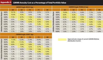
If we can calculate the net present value of the benefit for a GMWB annuity (Figure 2), what is the “cost” of insurance? The cost of purchasing a GMWB annuity will be reflected primarily in a smaller expected account balance at death because of the higher fees associated with the GMWB annuity as well as the different equity allocations in the approaches. This concept is reflected in Figure 3 for a male annuitant based on the same scenario in Figure 2 (although for a single retiree versus 100,000 retirees).
The amount the GMWB annuity beneficiary receives at death will vary based on when the annuitant actually dies. The longer the annuitant lives, the greater the expected difference in the account balances at death because of the effects of compounding (in other words, the greater the cost). The differences should be adjusted by expected mortality to determine the amount the annuitant can actually expect to receive, though. For example, while the difference in account balances in Figure 3 at age 90 is approximately $500,000, the probability of dying at age 90 is 3.64 percent. Note that 3.64 percent is not the probability of living to age 90; it is the probability of a retiree dying when he or she is 90 years old. Therefore, the actual “loss” the retiree is expected to experience in future dollars is $18,200 ($500,000 5 3.64 percent = $18,200). This same calculation would be performed for each retirement year to determine the mortality-weighted differences, and the net present value of all the mortality-weighted differences would be the total cost.
The discount rate for the net present value calculation is the compounded return of the 50 percent equity portfolio (6.57 percent). The discount rate for the cost calculation is higher than the discount rate used to calculate the GMWB benefit because the actual differences in the account values are subject to materially more variability than the income. Note that the range of account differences is neither constant nor guaranteed like the annuity income, so a higher discount rate is required. Also, the author contends the resulting account balance is worth less to the retiree than the income stream, which would warrant a higher discount rate. The cost estimate for each scenario is the net present value of the future expected account balances at death for the two approaches (how much less is expected to be in the GMWB portfolio versus the taxable portfolio). These cost figures for each of the scenarios in Table 1 are included in Appendix 2.
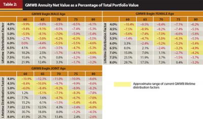
After the total expected benefits and total expected costs from the GMWB annuity have been calculated, it is possible to determine the net value of the GMWB annuity to a retiree. The net value is just the net present value of the expected additional cash flows minus the net present value of the expected decrease in the account value due at death to the additional costs associated with the GMWB annuity. These net value figures are included in Table 2 as a percentage of the initial investment in the GMWB annuity. As a reminder, because an annuity is a form of insurance we should not expect it to pay off on average; therefore, it should compare unfavorably to non-annuity portfolios in “average” scenarios. The objective of this paper is to provide the reader a better understanding of the components of cost-benefit analysis of the GMWB annuity.
The cost of the GMWB annuity, from the perspective of lost potential appreciation received by the annuitant’s heirs in today’s dollars in the taxable account, averages 6.5 percent for males, 6.1 percent for females, and 7.4 percent for couples, given current lifetime distribution factors. It may surprise the reader that the couple experienced higher relative costs (lowest net value) compared with males and females. At first someone might think the couple should receive the largest benefit because of having the longest life expectancy. However, the loss of potential capital appreciation in the taxable account versus the GMWB annuity outweighs the additional potential income for the couple.
Based on a lifetime distribution factor of 5 percent for a 65-year-old, the net cost of a GMWB annuity would be –8.1 percent for males, –7.4 percent for females, and –8.4 percent for a couple. Rates would need to improve by around 100 bps for the net value to equal the expected cost. In order for the net value of the GMWB annuity to be zero from an annuitant’s perspective (comparing the information in Table 2 to Table 1), the probability of actually using the GMWB annuity should be approximately 20 percent, although this varies materially by scenario. Therefore, if a financial planner is basing lifetime income amounts and decisions on probabilities of failure of less than 20 percent (for example, a 95 percent probability of success), a GMWB annuity should be considered for at least some portion of the portfolio.
Let’s Be Practical
The purpose of this analysis was to provide the reader useful insights about the expected value (or really the expected costs) of a GMWB annuity. Other options can be used to guarantee lifetime income as well, such as longevity insurance or immediate annuities. Just because the overall expected net value of a longevity protection strategy is negative does not mean it does not offer a valuable benefit to a retiree. The “cost” of any insurance product should be expected to be negative; the key is determining whether the aggregate benefits from the coverage, which are difficult to quantify, are worth the cost.
Someone thinking about using a GMWB annuity isn’t likely only focused on the “average” outcome, which was calculated in this study. He or she would likely seek to eliminate the “tail risk” associated with outliving his or her resources. Most financial planning professionals do not assume median life expectancies when developing a retirement income plan for their clients. Instead, financial planners typically use more conservative assumptions to minimize the probability of their clients running out of money during their lifetimes (they incorporate additional “costs” from a retirement income perspective to minimize the likelihood of retirement income failure).
Two scenarios that would increase the value of the GMWB rider to a retiree include: if the retiree (or adviser) expects market returns to be low during retirement, and if the retiree has a greater life expectancy than standard life expectancy tables predict. The value of the GMWB rider increases with lower returns because of the guaranteed income floor that doesn’t exist in a non-annuity taxable portfolio. Regardless of what happens to the annuity value, an annuitant is guaranteed lifetime income with a GMWB rider. Given that the “value” of the GMWB rider usually isn’t experienced until later in retirement (when the taxable portfolio would have run out of money), the longer a retiree lives, the greater its potential value.
Conclusion
A GMWB annuity rider is only going to “pay off” if two things happen: first, if the portfolio can no longer sustain the guaranteed withdrawal rate, and second, if the annuitant is still alive. The goal of this paper was to quantify the actual net value of a GMWB rider for male, female, and couple scenarios based on standard provisions of GMWB annuity contract provisions. The benefit an annuitant receives with a GMWB annuity rider is guaranteed lifetime income should the portfolio “fail” while the annuitant is still alive, while the cost is the lower projected balance transferred to the annuitant’s beneficiary upon death.
The analysis conducted for this paper suggests that the probability of a retiree actually needing income from a GMWB annuity, versus the income that could be generated from a taxable portfolio with the same value, is approximately 3.4 percent for males, 5.4 percent for females, and 7.1 percent for a couple, given current prevailing lifetime distribution factors (or guaranteed withdrawal rates). However, the net “cost” of the GMWB annuity from the perspective of the annuitant as a percentage of annuity total value is approximately 6.5 percent, 6.1 percent, and 7.4 percent of the initial portfolio value for males, females, and couples, respectively (again, given current lifetime distribution factors for GMWB annuities).
Because an annuity is a form of insurance, it would not be expected to have a positive average expected value, and will therefore compare unfavorably to non-annuity portfolios in “average” scenarios. The real question for a retiree is whether expected benefits are greater than or equal to the cost of the insurance. Based on the results of this study, the guaranteed income protection in a GMWB annuity may be a relatively inexpensive form of “longevity insurance,” especially from a behavioral finance perspective, as retirees greatly fear outliving their retirement income. Although the current guaranteed-rate environment is not generally favorable from an absolute average net value perspective, the author contends that GMWB-type features hold significant promise and that they are a viable strategy for managing longevity risk for a retiree.
References
Blanchett, David M., and Brian C. Blanchett. 2008a. “Data Dependence and Sustainable Real Withdrawal Rates.” Journal of Financial Planning 21, 9 (September): 70–84.
Blanchett, David M., and Brian C. Blanchett. 2008b. “Joint Life Expectancy and the Retirement Distribution Period.” Journal of Financial Planning 21, 12 (December): 54–60.
Chen, Peng. 2007. “Retirement Portfolio and Variable Annuity with Guaranteed Minimum Withdrawal Benefit (VA+GMWB).” http://corporate.morningstar.com/ib/documents/MethodologyDocuments/IBBAssociates/VA_GMWB.pdf.
Chen, Peng. 2011. “The Real Flaws: A Response to ‘Understanding Variable Annuities with GMWBs.’” www.advisorperspectives.com/newsletters11/The_Real_Flaws-A_response_to_Understanding_Variable_Annuities_with_GMWBs.php.
Huebscher, Robert. 2011. “Understanding Variable Annuities with GMWBs.” www.advisorperspectives.com/newsletters11/Understanding_Variable_Annuities_with_GMWBs.php.
Pfau, Wade D. “An International Perspective on Safe Withdrawal Rates from Retirement Savings: The Demise of the 4 Percent Rule?” Journal of Financial Planning 23, 12 (December): 52–61.
Milevsky, Moshe A. 2007. “Asset Allocation and Guaranteed Living Benefits in Variable Annuities.” http://www.advisorperspectives.com/newsletters11/Understanding_Variable_Annuities_with_GMWBs.php.
Xiong, James X., Thomas Idzorek, and Peng Chen. 2011. “Allocation to Deferred Variable Annuities with GMWB for Life.” Journal of Financial Planning (February): 42–50.