Journal of Financial Planning: January 2022
Executive Summary:
- The intent of this paper is to help financial advisers prepare for a client discussion about the required minimum distributions (RMD) withdrawal strategy, which many Americans follow.
- Clients who plan to follow this strategy need to be advised that the asset allocation they choose affects the volatility in the RMDs.
- It also affects the expected total number of dollars paid out over a client’s retirement life expectancy.
- Based on historic returns, the tradeoff between the volatility in RMDs and the expected number of dollars paid out is examined.
Stephen J. Larson, Ph.D., CFP®, is a professor of finance at Ramapo College of New Jersey. He teaches financial planning and insurance planning in addition to corporate finance. The main focus of his research has been in the area of financial planning.
NOTE: Please click on the images below for PDF versions.
JOIN THE DISCUSSION: Discuss this article with fellow FPA Members through FPA's Knowledge Circles.
FEEDBACK: If you have any questions or comments on this article, please contact the editor HERE.
To address the fear of running out of money during retirement, some retirees may plan on taking only their required minimum distributions (RMDs). However, this approach has its drawbacks, namely the volatility of the distributions. Clients who plan on taking RMDs should be encouraged to seek financial advice since the asset allocation they choose will not only affect the volatility of their distributions, but also the total number of dollars paid out from their retirement plan.
The main purpose of this study is to examine how asset allocation affects the tradeoff between the volatility in the RMDs and the expected number of dollars paid out. This is accomplished using historical Ibbotson data (Ibbotson and Harrington 2021). Financial advisers may elect to replicate the work done in this study to help prepare themselves for a discussion with clients who plan on taking RMDs. When doing this, they can accommodate estimates of the specific money management fees their clients would encounter.
Table 1 depicts a new retiree with a $2 million balance in a qualified retirement plan. It assumes they will take only their RMDs, and it assumes their asset allocation is 50 percent intermediate-term government bonds and 50 percent U.S. large-cap stocks. A 30-year retirement life expectancy is used. Finally, the bond and stock returns are expected to be the same as they were during a recent 30-year period (i.e., 1991–2020).
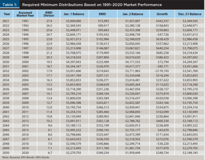
Several points can be made by reviewing Table 1. First, the initial distribution is $72,993 and the final distribution is $340,254, representing a 5.27 percent average annual increase [($340,254 / $72,993)1/30 – 1] in the RMD. Second, the balance in the account at the end of the 30-year period is $2,188,183. This amount can support further distributions if the client is still alive (i.e., longevity risk), or it will be available for heirs including charities (i.e., legacy planning) if they die. Third, the total number of dollars paid out is the sum of the RMDs plus the account balance at the end of the 30-year period, which comes to $9.2 million.
Unlike annuity distributions or the distributions that follow the 4 percent rule, the RMDs in the table are quite volatile. To illustrate, the second distribution ($89,417) is 22.5 percent higher than the first distribution ($72,993). The largest increase (i.e., 26.63 percent) in the distribution occurs between the fifth and sixth year while the largest decrease (i.e., 14.03 percent) in the distribution occurs between the 18th and 19th year. This is much different than Social Security benefits and distributions following the 4 percent rule, which are each adjusted year-to-year in order to maintain a steady stream of real income.
The RMDs will change if we assume market returns will follow the returns earned in a different historical period such as 1926 through 1955. More importantly, it will be shown that the variation in the RMDs along with the total dollars expected to be paid out are each dependent on the asset allocation.
Literature Review
Many Americans own individual retirement accounts (IRAs), and a number of these accounts are the result of rollovers from defined contribution plans. According to Mortenson, Schramm, and Whitten (2019), total IRA wealth rose to about $9.5 trillion in 2018, and this represents about one-third of total retirement assets in the United States. Moreover, in 2015, about 40 million households held at least one IRA. Finally, in 2018, the federal government spent $17.8 billion (i.e., forgone tax revenue) in order to encourage Americans to save.
Two recent studies suggest more than half of retirees opt to collect RMDs instead of following another approach such as the 4 percent rule. First, according to Fortuna (2019), more than half of the clients who funded their traditional IRAs with Fidelity Investments were taking only their RMDs. Second, Barney (2018) referred to an Ameriprise survey of more than 1,000 retirees who had at least $100,000 in investable assets. A key conclusion of Barney’s research was that 68 percent of these retirees were taking only their RMDs.
There is evidence that retirees who have adopted another strategy, such as the 4 percent rule, are actually taking their RMDs by default. Larson (2018) examined the impact of RMDs on the 4 percent rule by using past returns to model withdrawals from a $1 million retirement account over the next 30 years. Specifically, when the RMD exceeded the planned withdrawal, he assumed the RMD was taken in order to avoid the tax penalty. For a portfolio composed of 60 percent stocks–40 percent bonds, the RMDs exceeded the planned distribution 67 percent of the time. This suggests that many retirees who planned on following the 4 percent rule are actually taking their RMDs most of the time. Mortenson et al. (2019) used a nationally representative panel of 1.8 million IRA holders from 2000 to 2013. They claimed that about 50 percent of the people surveyed would have rather withdrawn amounts less than their RMDs. They also claimed that about 62 percent of retirees took advantage of the temporary suspension of RMD rules in 2009. These two studies suggest that many retirees follow the RMD strategy of withdrawals simply because they have to in order to avoid the 50 percent penalty tax.
The RMD strategy may appeal to retirees because, unlike other strategies (e.g., the 4 percent rule), it is a dynamic withdrawals strategy (Sun and Webb 2012). As a retiree ages, the RMD divisor becomes smaller, so a larger percent of wealth is distributed in line with the reduction in their life expectancy. That is, RMDs are actuarily based. Moreover, the distributions year to year respond to market conditions, meaning, for example, a stock market decline one year will translate into a smaller RMD the next. The 4 percent rule, in contrast, ignores this. Its next year’s distribution is based only on two things: this year’s distribution and this year’s inflation rate. Moreover, the RMD strategy is easy to follow. That is, in order to determine this year’s distribution, the retiree simply divides last year’s ending retirement plan balance by the age-appropriate divisor in a government table.
According to Benz (2019), following a strategy of collecting RMDs can make budgeting difficult. Large swings in market returns can translate into significant disruptions in the annual distributions, and this may cause financial distress in a household.
The main purpose of this research is to demonstrate just how asset allocation affects both the expected volatility of the RMDs as well as the expected number of dollars paid out from a retirement plan.
The Nature of Required Minimum Distributions
Clients who feel they don’t need professional financial advice on taking RMDs from a qualified retirement plan may be making a big mistake. First of all, they need to be made aware of how RMD volatility will affect their household budget year to year. More importantly, however, they will need assistance in choosing an asset allocation after being shown its role in determining RMD volatility and the total number of dollars paid out over their retirement life expectancy.
Collecting RMDs from a qualified plan is quite a bit different than collecting the stream of distributions that arise from following a distributions rule such as the 4 percent rule. With the 4 percent rule, the distributions are designed to keep up with inflation. For example, if this year’s distribution is $73,000 and inflation runs at 2.5 percent, then next year’s distribution will be $74,825. This enables clients to enjoy a stable pattern of distributions, one that leaves their purchasing power intact. Of course, Social Security benefits are adjusted for inflation in the same manner.
A typical example of a decline in a retirement portfolio’s yield points out the consequences of RMD volatility. For instance, the market may decline by 20 percent during the first year of retirement. Given $2 million at retirement, the first distribution at the beginning of the year would be $72,993 (i.e., $2,000,000 / 27.4) leaving $1,927,007 in the account. At the end of the year, the account balance would be $1,541,606 given the 20 percent market decline. The year-two RMD would be based on this amount, resulting in a distribution of $58,174 (i.e., $1,541,606 / 26.5), representing a decline in the distribution of 20.3 percent. Given that inflation runs at 2.5 percent the first year of retirement, the second distribution would have been $74,818 if they had followed the 4 percent rule instead. Naturally, the degree of volatility would be higher if a more aggressive asset allocation was used.
Another issue clients should be made aware of is the tradeoff between expected RMD volatility and the total number of dollars expected to be paid out from a retirement account. Past market performance suggests that if a retiree can settle for a higher degree of RMD volatility, more money will flow from their account if they select a portfolio more heavily weighted in stock. This tradeoff is examined below.
Data and Method
Using historical average bond and stock returns (i.e., point estimates) to project retirement balances can lead to a false sense of security since market volatility matters. To illustrate, suppose markets decline by 20 percent the year a person retires with $2 million and that they take an $80,000 distribution the day they retire. This would leave them with only $1,536,000 [($2,000,000 – $80,000) × (1 – 0.20)] at the end of the year. That is, their retirement balance at the end of the first year of retirement is 23 percent lower than it was at the beginning of the year. Of course, 4 percent ($80,000) of the decline is due to the distribution. Had we modeled their distributions using an 8 percent expected return (i.e., point estimate) instead of a 20 percent decline, the projected end-of-the-year balance would be $2,073,600 [($2,000,000 – $80,000) × 1.08].
Bierwirth (1994) used overlapping samples of historical returns to project future retirement plan balances. The purpose was to account for variation in market (i.e., bond and stock) returns as well as inflation. Following Bierwirth’s approach, historical returns for bonds and stocks are used to project the retirement account balance for a retiree who plans on taking RMDs. The asset allocation is controlled for; specifically, 21 asset allocations (0 percent bonds, 5 percent bonds, 10 percent bonds . . . 100 percent bonds) are examined.
Ibbotson total returns data for the period 1926 through 2020 are used for a retiree who retires with $2 million in their qualified retirement plan. It is assumed they will follow a strategy where they will withdraw their RMDs at the beginning of each year. This retiree plans for a 30-year retirement period in case they live that long. Therefore, 30 years of retirement distributions are projected. Following Bengen’s (1994) popular study, “Determining Withdrawal Rates Using Historical Data,” the bond return series represents intermediate-term government bonds, and the stock return series represents the S&P 500 index.
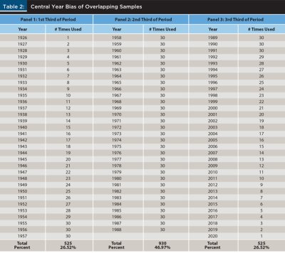
There is an issue with using overlapping samples; they favor data occurring in the middle of the sample period. Table 2 illustrates the central-year bias inherent in using the overlapping samples. Ninety-five years (1926–2020) of data are available from Ibbotson and Harrington (2021). In the first run, bond and stock returns for the years 1926–1955 are assumed to repeat themselves during the next 30 years (i.e., 2021–2050). In the second run, the returns for 1927–1956 are assumed to repeat themselves during the next 30 years, and so on. Notice that 1926 drops out in the second run, and the years 1927–1955 are used a second time. The effect of using these overlapping samples is to favor the years in the middle of the sample period.
In Table 2, the sample period (i.e., 1926–2020) is broken down into three approximately equal sub-periods (i.e., 1926–1957, 1958–1988, and 1989–2020). The years in the middle of the period are used 930 times whereas the years in each of the other two sub-periods are used only 525 times. So, the bond and stock returns during the middle one-third of the sample period account for nearly half [i.e., 930 / (525 + 930 + 525) = 0.47] of the data used to forecast the performance of the example portfolio from which RMDs will be taken.
Results
Table 3 depicts the historic tradeoff between RMD variability and the total dollars paid out over a 30-year period for 21 different asset allocations (i.e., 0 percent bonds–100 percent stocks, 5 percent bonds–95 percent stocks, 10 percent bonds–90 percent stocks . . . 100 percent bonds–0 percent stocks).
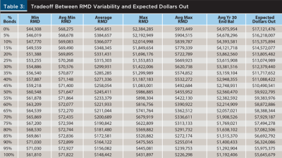
The first row inside the table depicts the outcome when the portfolio is assumed to be composed of 0 percent bonds. Like the other rows, it reflects the outcome of 66 runs. In the first run, the stock returns for the period 1926–1955 were used, and in the second run, the years 1927–1956 were used. In the final (66th) run, the returns for years 1991–2020 were used. Given a 30-year retirement life expectancy and 66 runs, the total number of estimated RMDs represented is 1,980.
For the 0 percent bonds portfolio, the smallest RMD out of the 1,980 estimated RMDs is $44,308. The average minimum RMD across the 66 runs is $68,275, and the average RMD across all 1,980 RMDs is $404,851. The maximum RMD out of all 1,980 RMDs is $2,384,285 whereas the average maximum RMD across the 66 runs is $973,449. So, using past data, the worst-case RMD is $44,308 and the RMD averaged $404,851 over the 30-year period.
The seventh column depicts the average ending (i.e., Year 30) retirement account balance. For the 0 percent bond portfolio, this amount is $4,975,954. The final column (i.e., Column 8) depicts the expected number of dollars to be paid out. It is the average RMD times 30 plus the expected year-30 ending balance. So, for the 0 percent bonds portfolio, one can expect a client to collect $12,145,530 (i.e., 30 years × $404,851) in RMDs plus have $4,975,954 remaining in the account at the end of the 30-year retirement life expectancy. Therefore, the expected number of dollars paid out is about $17.1 million.
The results for the remaining asset allocations (i.e., 5 percent bonds–95 percent stocks to 100 percent bonds–0 percent stocks) can be examined in Table 3.
Implications for Advisers
So, how would an adviser explain the 0 percent bonds portfolio to a retiring client who is planning on taking RMDs from their qualified plan? First of all, the client should understand the discussion is based on prior (i.e., 1926–2020) bond and stock returns and that worse scenarios may occur in the future. They should also understand that the results are based on total returns, which are not adjusted for money management fees. The adviser could then tell them the first RMD will be $72,993, which is the $2 million balance divided by the RMD divisor (i.e., 27.4). Clients should understand that future distributions will be based on the divisor, which declines over time, and the future performance of the bonds and stocks they hold. Of course, they should be made to understand that, unlike Social Security benefits and pension benefits, RMDs can be quite volatile.
Looking at Row 1 inside the table, clients should understand that their RMD is expected to average $404,851 during the 30-year period, but expect it to decline to a minimum of $68,275 and rise to a maximum of $973,449. However, based on past market movements, the RMD may be as low as $44,308 one year and as high as $2,384,285 in another year. The client may wonder about living longer than 30 years or they may have legacy planning goals. According to the analysis, their expected account balance will be $4,975,954 at the end of the 30th year. Finally, the total RMDs plus the ending balance is expected to total $17,121,476.
As the client and adviser work their way down the table, more bonds (fewer stocks) are used in the portfolio. The minimum RMDs rise as do the average minimum RMDs. However, the average RMDs decline along with the average year-30 ending balances and the expected number of dollars to be paid out. This depicts the tradeoff. As the client adds more bonds into their portfolio, the RMDs are less volatile, yet fewer dollars are expected to be paid out during the 30-year retirement life expectancy.
Once a client studies the table with their adviser, they can choose their ideal asset allocation. A client who needs the distributions for non-discretionary expenses may choose the 30 percent bonds (70 percent stocks) asset allocation if they feel an RMD substantially below $55,000 is unacceptable. Their RMDs are expected to average $299,931, and they are expected to have about $3.4 million dollars remaining at the end of the 30-year retirement life expectancy. The total expected dollars received from the plan is about $12.4 million.
A client who plans to use the $2 million in this account for discretionary items (e.g., entertainment and vacations) may choose the 0 percent bond (100 percent stock) portfolio. They may reason that a bad year would not hurt them too much since they consider it their “fun” money. They could expect an average RMD of $404,851, an ending balance equal to $4,975,954, and a total number of dollars paid out of $17,121,476.
It is interesting to note the importance of having at least some stock in a portfolio heavily weighted in bonds. Referring to Column 2 (i.e., Min RMD) of Table 3, as more bonds are added to the portfolio, the minimum RMD steadily rises. However, for the last entry (i.e., 100 percent bond portfolio), the minimum RMD drops substantially. Specifically, the minimum RMD for the 100 percent bond portfolio is $9,220 (i.e., $71,030 – $61,810) less than for the 95 percent bond portfolio. This suggests the “lift” from at least some stock is crucial for downside protection when constructing a portfolio heavily weighted in bonds.
This paper does not advocate for one withdrawal strategy over any of the others. It simply acknowledges that many retirees follow the RMD strategy, and as a consequence need to be advised on how their asset allocation will affect the volatility of their RMDs and the total dollars expected to be removed from the plan.
Conclusion
The purpose of this paper is to help financial advisers prepare for a discussion with clients who plan on taking RMDs from a qualified retirement account such as a 401(k) plan or traditional IRA. Clients should understand that these distributions tend to be quite volatile and that the volatility depends on their asset allocation. It is important for them to understand the tradeoff between RMD volatility and the total expected number of dollars paid out during their retirement life expectancy.
Citation
Stephen Larson. 2021. “Required Minimum Distributions as a Retirement Strategy: The Tradeoff Between RMD Volatility and the Expected Number of Dollars Paid Out.” Journal of Financial Planning 35 (1): 60–67.
References
Barney, Lee. 2018, June 21. “Most Retirees Only Withdrawing Required Minimum Distribution.” PlanAdviser. www.planadviser.com/retirees-withdrawing-required-minimum-distribution/.
Bengen, William P. 1994. “Determining Withdrawal Rates Using Historical Data.” Journal of Financial Planning 7 (4): 171–180.
Benz, Christine. 2019, March 7. “Should Your Withdrawals Mirror Your RMDs?” Morningstar. www.morningstar.com/articles/918416/should-your-withdrawals-mirror-your-rmds. Accessed February 16, 2021.
Bierwirth, Larry. 1994. “Investing for Retirement: Using the Past to Model the Future.” Journal of Financial Planning 7 (1): 14–24.
Fortuna, Nick. 2019, December 12. “4 Ways to Manage Your Required Minimum Distributions When You Don’t Need the Money.” Barron’s.
Ibbotson, Roger G., and James P. Harrington. 2021. 2021 SBBI® Yearbook: Stocks, Bonds, Bills, and Inflation®. New York, NY: Duff & Phelps, LLC.
Larson, Stephen J. 2018. “Strategy: Assessing the Impact of RMDs on the 4 Percent Rule.” Journal of Financial Service Professionals 72 (1): 55–63.
Mortenson, Jacob A., Heidi R. Schramm, and Andrew Whitten. 2019. “The Effects of Required Minimum Distributions Rules on Withdrawals from Traditional IRAs.” National Tax Journal 72 (3): 507–542.
Sun, Wei, and Anthony Webb. 2012. “Can Retirees Base Wealth Withdrawals on the IRS’ Required Minimum Distributions?” Center for Retirement Research at Boston College. Issue Brief 12 (19).