Journal of Financial Planning: January 2017
Sherman D. Hanna, Ph.D., is a professor in the Human Sciences Department of The Ohio State University. He received a bachelor’s degree in economics from the Massachusetts Institute of Technology and a Ph.D. in consumer economics from Cornell University. He has published in numerous journals and was the founding editor of the Journal of Financial Counseling and Planning.
Kyoung Tae Kim, Ph.D., is an assistant professor in the Department of Consumer Sciences at the University of Alabama. He received a bachelor’s degree in economics and a Ph.D. in consumer sciences from The Ohio State University, and a master’s degree in economics from Purdue University. He has published in Applied Economics Letters, Financial Services Review, Journal of Poverty, and Journal of Personal Finance.
Executive Summary
- The typical treatment of inflation in retirement planning textbooks is complex and often not reasonable in terms of the amount to contribute, the first year being dependent on the inflation rate assumption.
- The typical financial planning approach requires an assumption about the future inflation rate, which can be difficult to justify based on the economic history in the United States and other countries.
- Economists typically put all amounts and interest rates in inflation-adjusted terms, which is simpler and can be a more rational approach to long-term planning.
- It can be difficult to comprehend the meaning of future amounts in nominal terms; therefore, doing projections in inflation-adjusted terms may help clients better understand projections.
- In calculating the capital needs for retirement, inflation-adjusted rates of return for each step should be chosen based on portfolio choices appropriate for before and after retirement.
A review guide for the Certified Financial Planner™ examination includes the following statement: “The client needs to make an assumption regarding the effects of inflation during the period necessary to accumulate assets, as well as during the distribution phase in retirement” (Keir 2009, page 59.2). This statement is consistent with the methods presented in a number of financial planning and retirement planning textbooks, but it assumes expertise on the part of the client, and therefore may be unreasonable. It is also part of what may be considered a convoluted calculation method that is not consistent with analyses by economists. The pattern of contributions relative to income derived by this method depends on the inflation rate assumed, in ways that make little economic sense.
The purpose of this article is to show that inflation is not properly discussed in financial planning and retirement planning textbooks and in the CFP® examination, and that the calculation method presented in these textbooks is not consistent and may lead to unreasonable recommendations for clients. This article presents a simpler method that leads to more reasonable results, and is consistent with the approach taken by economists.
Overview of Inflation
Inflation is the change in overall prices for goods and services. In the United States, the most commonly used measure of inflation is the Consumer Price Index (CPI), which tracks the weighted average of prices of many consumer goods and services (McGinty 2015). Economists have found that if the rate of inflation increases, nominal interest rates will usually increase correspondingly (Bodie, Kane, and Marcus 2009, page 129). This idea was articulated by economist Irving Fisher in 1930 (as discussed in Mishkin 1992), and according to Mishkin, the Fisher effect tends to hold in the long run. Therefore, economists typically use real (inflation-adjusted) rates and dollar amounts in analyses. The standard presentation of the normative life cycle model (e.g., Hanna, Fan, and Chang 1995) has every amount and rate in inflation-adjusted terms, because the theoretical basis of the theory is maximization of the utility of real consumption over one’s lifetime.
The optimal percent of income to save in a particular year should depend on the real pattern of income in the future, present assets, and real interest rates—not on the rate of inflation. Economists analyzing optimal saving for retirement, e.g., Ibbotson Associates (2015, pages 164–166), put all rates and amounts in inflation-adjusted terms. Empirical analyses of retirement adequacy, which include calculation of how much capital households need at retirement, use inflation-adjusted rates of return on investments, and all amounts are in inflation-adjusted terms (e.g., Munnell, Webb, and Golub-Sass 2012; Scholz, Seshadri, and Khitatrakun 2006).
Retirement planning textbooks generally present a mixed method with nominal interest rates and nominal amounts of income needs. Thinking about prices and interest rates in nominal terms can be challenging. For instance, current movie box office receipts are very high in nominal terms, but the all-time highest grossing movie in U.S. box office receipts in real terms, “Gone with the Wind,” had only $198 million in receipts in nominal terms in 1939 (Schwartzel 2015), so that box office flops released today usually have far higher nominal receipts than the 1939 movie.
If inflation remains low, it will not be too challenging to think about amounts in nominal dollars 10 years in the future, but for a young worker, nominal amounts during retirement would likely be difficult to comprehend. For very long time periods, the nominal accumulations possible with financial investments can be misleading to average people. For instance, a one-time investment of $1,000 in a hypothetical small stock index fund on December 31, 1925 would have accumulated to $26,433,350 in nominal terms by December 31, 2015, but only $1,994,300 in inflation-adjusted terms (Ibbotson 2016, pages 4–7).
What is a reasonable inflation rate to assume for the future? The natural tendency among consumers and economists is to assume that recent trends will continue. Over the period 1914 to 2015, the arithmetic mean inflation rate in the U.S. was 3.2 percent per year, and the annual rates ranged from a low of –10 percent to a high of 20 percent.1 The periods of very high inflation have been related to wars and energy crises: World War I, World War II, the Vietnam War, and energy shocks in the 1970s. In most of the past 50 years, some countries experienced very high inflation and other countries experienced deflation. In 2007, annual inflation rates in the World Bank database ranged from –10 percent to 35 percent.2
Figure 1 shows the U.S. inflation pattern for the period 1965 to 2015, with the annual change in inflation, the five-year moving average, and the mean rate over the period (4.1 percent). Over the period 1926 to 2015, the arithmetic mean of inflation was 3.0 percent per year, but the highest mean rate for a 10-year period was 8.7 percent per year for the period ending in 1982 (Ibbotson 2016).
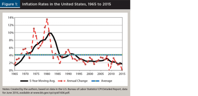
Expectations for future inflation are influenced by recent patterns. In a Delphi survey of financial planners and educators, Greninger, Hampton, Kitt, and Jacquet (2000) found general agreement that an inflation rate of 4 percent per year should be used for retirement planning, a rate roughly equal to the five-year moving average at the time of the survey. It is plausible that a similar survey in 1983 would have had a much higher consensus inflation rate, perhaps near the five-year moving average of 9 percent. Since the year 1992, the inflation rate has been below 4 percent, and the five-year moving average as of 2015 was 1.7 percent.
What factors are related to the inflation rate? Over the long run, a nation’s inflation is the result of political decisions, and one motivation to push the inflation rate higher is the belief that somewhat higher inflation can increase employment. Phillips (1958) proposed what became known as the Phillips Curve (Phelps 1967), and even though there is controversy over the validity of the relationship (Lansing 2002), the idea persists among many economists that moderate inflation, e.g., 2 percent per year, is better for employment than inflation rates lower than 2 percent. As with stimulants for people, though, there is general agreement that high inflation rates would likely cause more harm than good.
Why might a government let the inflation rate increase? In addition to the idea that more inflation might stimulate the economy, the existence of a large national debt could lead to pressures to let inflation increase. To the extent that an income tax system is not indexed to inflation, increases in the inflation rate will bring in more revenue without a direct increase in income tax rates. For instance, with low inflation rates, taxes received from capital gains are relatively low, but with high inflation, capital gains will be much more heavily taxed (Aaron 1976).
A country might also let inflation increase to ease the burden of paying down the national debt, especially if a high proportion of the debt is held by foreigners. Aizenman and Marion (2011) suggested that increasing the U.S. inflation rate to 5 percent per year could help reduce the burden of the federal debt at the expense of holders of the debt in China, Japan, and other countries. Such policies have long-term costs, and perhaps it is unlikely that political turmoil in the United States would lead to inflation rates being persistently higher than the 2 percent to 3 percent range of the 1995 to 2016 period, but it is possible. Analysis of inflation rates around the world3 shows that of 180 countries with inflation rates reported for the period 1995 to 2014, more than 24 percent had mean inflation rates for that period of 10 percent per year or higher. The maximum 20-year mean was 412 percent per year, and even some countries in Europe had mean rates higher than 25 percent per year.
Optimal Retirement Planning
This article focuses on the method used in retirement planning textbooks to calculate the capital needed at retirement. What is the optimal way to do this in terms of economic theory? The normative life cycle model (Hanna, Fan, and Chang 1995; Hanna 2010) implies consumption smoothing, which implies that for workers with increasing income, it may be optimal to have low or even negative saving out of income early in the life cycle. The goal is assumed to be to maximize the expected lifetime utility from consumption, and the interest rate or rate of return faced by the household is one important element in the optimization, but the worker’s personal discount rate is also important. For advice to workers, it may be plausible to calculate optimal saving patterns based only on discounting for the risk of death (Hanna and Kim 2014), but workers might have higher discount rates based on impatience and expectations of changing household situations.
As Hanna and Kim (2014) noted, many normative analyses by economists have used relatively high personal discount rates. If a high personal discount rate is reasonable, then low saving when young may be rational. In terms of the focus of this article, it is important to note that economists considering optimal saving over the life cycle specify all income and consumption amounts and interest rates in inflation-adjusted terms, so the level of inflation should not affect the optimal pattern of saving.
Treatment of Inflation in Textbooks
The standard treatment of inflation in financial planning textbooks used to prepare students for the CFP® examination is to assume an inflation rate to inflate income needed at retirement to the nominal dollar amount in the year of retirement, assume a nominal rate of return on investments, calculate an inflation-adjusted rate of return during retirement to find the capital needed for retirement, then use the nominal rate of return on investments to calculate how much needs to be contributed to a retirement fund each year before retirement (e.g., Dalton and Dalton 2016).
Retirement planning software programs generally follow similar methods with assumptions about nominal rates of return, inflation, etc., or provide users the opportunity to input values for some parameters (Bi 2015; Dorman, Mulholland, Bi, and Evensky 2016).4
Although some authors have advocated a consistent approach, suggesting that nominal and real rates of return should not be mixed in analyses (e.g., Joyce 2000), financial planning textbooks currently used to prepare students for the CFP® examination use a method that requires assumptions about nominal rates of return and inflation.
A detailed example is shown below, generally following the methods presented in Dalton and Dalton (2016) and other retirement planning textbooks. This “standard” approach has several problems, starting with the assumption of an inflation rate. A similar approach has been presented by a Consumer Reports guide for consumers to use a retirement calculator: “Inflation: input 3 or 3.5 percent. Pessimistic? Use 4 or 5 percent.”5
The idea that ordinary consumers can predict long-term inflation has no reasonable basis, considering that experts cannot predict inflation (Tutino 2015). The inflation expectations of both consumers and experts tend to lag actual inflation, and expectations have been substantially diverse at any particular time (Mankiw, Reis, and Wolfers 2003).
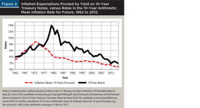
Figure 2 shows the patterns since 1962 of the nominal yield on 10-year U.S. Treasury notes, often assumed to reflect inflation expectations, and the arithmetic mean of annual inflation for the 10-year period starting with each current year. For instance, the 10-year nominal yield in 1981 was 13.9 percent, while the mean inflation rate for the period 1981 to 1990 was 4.7 percent. Although this is not a rigorous analysis, clearly the market expectations as reflected in the 10-year bond yield were often proven inaccurate.
Annuity Method
The basic method of calculating capital needs for retirement is equivalent to the assumption that at retirement, the worker purchases an inflation-adjusted life annuity with no residual amount left at death. Dalton and Dalton (2016, pages 46–49) refer to this as the “annuity method.” As will be shown below, the inflation rate assumed has a substantial effect on the recommended amounts to contribute to retirement funds.
Consider a simple case: a worker who just turned 25 years old plans to retire in 40 years and has a salary of $100,000 per year, which is expected to increase with inflation until retirement. Using the standard approach in financial planning textbooks, a wage replacement rate is chosen (for example, 80 percent), resulting in total income needed at retirement in today’s dollars of $80,000 per year. Income at retirement other than what would be generated by retirement investments is estimated in today’s dollars. Typically, this would be a Social Security pension, so assume a pension of $20,000 per year. The result is that at retirement, an income from retirement investments of $60,000 per year in today’s dollars is needed. The next step is to assume an inflation rate (for example, 3 percent per year), and apply that to the needed income in retirement so that in the first year of retirement, $195,722 of income is needed, as measured in nominal dollars. Following Dalton and Dalton (2016), income taxes are not explicitly considered to simplify presentation.
The next step is to calculate the present value of the income needed using an inflation-adjusted interest rate. With the annuity method (e.g., Dalton and Dalton 2016), a worker would plan to accumulate an amount of investments by retirement that would finance annual retirement income for the remaining life expectancy at retirement, or purchase a life annuity that would provide annual retirement income as long as the person lived. For the examples discussed below, an inflation-adjusted rate of 3 percent per year was assumed. With inflation assumed to be 3 percent, a nominal rate of return, 6.09 percent was used. Assuming a remaining life expectancy of 25 years and payments at the beginning of each year, the present value of $3,510,385 is the amount of capital needed the day of retirement to finance the withdrawals needed at the beginning of each year during retirement.
The final step is to calculate how much needs to be contributed each year until retirement. Some authors present calculations for monthly contributions (Dalton and Dalton 2016, page 48), but below, annual contributions were assumed. Assuming contributions at the end of each year for 40 years, and a nominal rate of return of 6.09 percent, $22,175 per year must be contributed for 40 years to reach the capital needed at retirement. Table 1 shows a spreadsheet for these calculations. Column B has the textbook approach, inflating the net needs at retirement to nominal dollars based on the inflation rate assumed. In this example, with a 3 percent inflation rate assumed (cell B11), and a 6.09 percent nominal rate of return (cell B15), the capital needed at retirement to provide an income of $195,722 per year is $3,510,385, and the worker would need to start contributing $22,175 at the end of each year for 40 years.
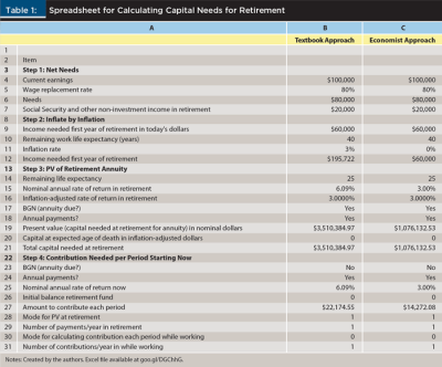
The effect of varying the inflation rate with the real rate of return constant. The textbook annuity method may seem reasonable, but an examination of varying the assumption about the inflation rate shows some flaws in the standard method. In Table 1, column C shows the “economist approach” with the same assumptions listed for the textbook approach, except using consistent inflation-adjusted calculations. For consistency in the spreadsheet, inflation is listed in cell C11 as 0 percent, but that is just in order to be able to compare calculations to the textbook approach. Obviously, Step 2 is not needed, as the amount of income to be generated the first year of retirement is the same as the constant dollar calculation. The capital needed at retirement with a 0 percent inflation rate, $1,076,133, represents the capital needed at retirement in today’s dollars. The amount the worker would need to start contributing each year would be $14,272 at the end of each year, with increases each year with inflation.
Figure 3 was calculated based on having the inflation-adjusted rate of return be equal to 3 percent for inflation rates varying from 0 percent to 7 percent. The higher nominal amounts of capital needed at retirement for higher inflation rates represent the same real amount, $1,076,133. At a 7 percent inflation rate, a nominal amount of capital of $16,114,501 would be needed at retirement.
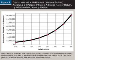
Figure 4 shows the amount to be contributed to the retirement fund at the end of each year for 40 years, by the assumed inflation rate, as a percent of the salary at age 25. With a 0 percent inflation rate, only 14 percent of the salary would need to be contributed, but with a 7 percent inflation rate, 34 percent of the salary would need to be contributed the first year. The percent to contribute at age 25 is based on the same inflation-adjusted interest rate, for inflation rates ranging from 0 percent to 7 percent.
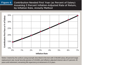
For inflation rates above 0 percent, the proportion of salary to contribute each year would decrease every year, as the nominal contribution would remain the same while the salary would increase with inflation. If the worker’s salary increased faster than inflation, the relative burden of the contribution would decrease even more substantially each year. This makes little sense in terms of typical life cycle patterns of households, and employer-defined contribution plans with defaults based on concepts of economic theory offer lower contribution rates to new workers (Thaler and Benartzi 2004). Younger workers may be paying off education loans, buying vehicles, furniture, and homes, and having children. The idea that the burden of contributing to a retirement account should be highest in real terms at a young age does not make sense for many younger workers, and this is recognized by Thaler and Benartzi. The fact that the first-year contribution with the standard approach is so dependent on the inflation rate assumed makes no sense in terms of economic theory. The normative life cycle model is based on the idea that consumption smoothing maximizes expected utility from consumption, and the optimal consumption pattern should depend on the real rate of return, not on the inflation rate (Hanna 2010).
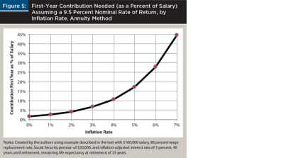
The effect of varying the inflation rate with the nominal rate of return constant. Figure 5 shows another example based on the standard approach in retirement planning textbooks. Assume a nominal rate of return on investments of 9.5 percent per year (Dalton and Dalton 2016, page 48), with other assumptions the same as the previous example. With an inflation rate of 2 percent per year, the worker would need to contribute more than 4 percent of the initial salary to the retirement fund. With an inflation rate of 7 percent per year, the worker would need to contribute almost 45 percent of the initial salary to the retirement fund. In each case, the nominal contribution to the retirement fund would remain constant based on the standard approach, resulting in decreasing real contributions during the worker’s career. The dependence of the first-year contribution on the inflation rate assumed makes sense in terms of higher inflation rates resulting in lower inflation-adjusted rates of return, but this example shows the potential problems due to separating assumptions about the nominal rate of return from assumptions about the inflation rate.
A more rational method would be to put every amount and interest rate in inflation-adjusted terms, similar to the approach used in Ibbotson Associates (2015, pages 164–166).
Using a Consistent Inflation-Adjusted Procedure
Putting every amount and interest rate in inflation-adjusted terms would produce results similar to those for the 0 percent inflation shown in Figures 3 and 4. In the example illustrated in Figure 3, the $1,076,133 needed at retirement would represent purchasing power as of today, so the target would be more understandable by clients. The first-year burden of contributing to a retirement fund would be more tolerable. Neither the client nor the planner would have to make an assumption about the inflation rate.
Some personal finance and financial planning textbooks present an inflation-adjusted approach (e.g., Garman and Forgue 2015, page 514; Mittra, Sahu, and Crane 2007, pages 11-5 and 11-6), but retirement planning textbooks used for courses aimed at preparing students for the CFP® examination, including Dalton and Dalton 2016, use the standard treatment described in the examples for Figures 3, 4, and 5. With a consistent inflation-adjusted calculation, historical real rates of return could be used rather than current nominal rates of return.
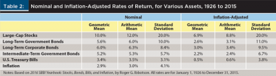
Table 2 shows nominal and inflation-adjusted mean rates of return for five categories of financial assets, plus inflation. In the mixed approach used in current retirement planning textbooks, one needs to choose an appropriate nominal rate of return (for example, the arithmetic mean rate of return for 1926–2015 for large stocks is 12 percent, and the arithmetic mean inflation rate for 1926–2015 is 3 percent.) For a consistent inflation-adjusted approach, one would need to only choose an appropriate inflation-adjusted rate of return (for example, 8.8 percent for large stocks), and there would be no need to assume a particular inflation rate.
For sensitivity analyses, it would be prudent to use pessimistic projections of rates of return (Dalton and Dalton 2016, pages 53–55.) For longer time periods, there are several approaches to calculate ranges of returns, including projections based on the assumption that returns have a normal distribution, and projections based on the assumption that returns have a lognormal distribution (Ibbotson 2016, page 10-2).
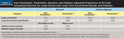
Table 3 shows very pessimistic and pessimistic projections of nominal and inflation-adjusted annualized returns for a 20-year horizon for large stocks and long-term government bonds, and also high and low projections of inflation rates based on the arithmetic means and the standard deviations shown in Table 2 and the assumption of normal distributions. (Projections based on the assumption of lognormal distributions are similar.)
For a period of N years, a projection based on the normal distribution starts with a calculation of the annualized standard deviation, which is the standard deviation based on one-year periods, divided by the square root of N (Ho, Perdue, and Robinson 1998, pages 265–270). For instance, the annualized inflation-adjusted standard deviation for 20-year periods for long-term government bonds is 11 percent/(200.5) = 2.5 percent. The annualized mean return for a probabilistic projection is the mean + (Z x S), where S is the annualized standard deviation, and Z is the value of the Z statistic corresponding to the portion of the normal curve we need to examine.
In Table 3, “very pessimistic” for investments is defined as the mean minus two annualized standard deviations (Z = –2), and “pessimistic” is defined as the mean minus one annualized standard deviation. A very pessimistic projection of the annualized inflation-adjusted rate of return for large stocks for 20-year periods is –0.1 percent, and a pessimistic projection is 4.3 percent. The range of estimates is the same for the nominal rate of return, because the annual standard deviation is the same, but if one used the textbook approach, then an estimate of inflation is also needed, with a very low estimate (mean minus two annualized standard deviations) of 1.2 percent, and a very high estimate of 4.8 percent. A very pessimistic projection of the annualized inflation-adjusted rate of return for long-term government bonds for 20-year periods is –1.8 percent, and a pessimistic projection is 0.6 percent. For comparison to the probabilistic projections, the lowest nominal annualized return for the 71 overlapping 20-year periods was 3.1 percent for large stocks and 0.7 percent for long-term government bonds (Ibbotson 2016, page 2-20). The lowest annualized inflation rate for 20-year periods was 0.1 percent and the highest rate was 6.4 percent.
To use a consistent inflation-adjusted approach to calculating the amount needed to save for retirement, the steps for the annuity method would be similar to the current method used in retirement planning textbooks, except that the planner or consumer would not need to assume a particular inflation rate.
Consider the first example presented in this article—a worker who just turned age 25, plans to retire in 40 years, and has a salary of $100,000 per year. If we assume that the salary will increase with inflation, then just before retirement the worker would have a real salary of $100,000 in terms of today’s prices. The amount of retirement income could be estimated in several ways, such as a budgeting approach (Dalton and Dalton 2016, pages 35–37), but we will use a wage replacement rate of 80 percent to be consistent with our previous example. The total income needed at retirement in today’s dollars would be $80,000 per year. Assume a Social Security pension of $20,000 per year. At retirement, an income from retirement investments of $60,000 per year in today’s dollars is needed. With the inflation-adjusted approach, there is no need to calculate the nominal amount of income needed the first year of retirement.
The next step, calculating the present value of the income needed, is the same as the standard approach, using an inflation-adjusted interest rate, presumably based on the average inflation-adjusted rate of return consistent with an appropriate portfolio or annuity. As with our first example, an inflation-adjusted rate of 3 percent per year is assumed, a remaining life expectancy of 25 years, and payments at the end of each year. (Note that it may be reasonable to assume a lower rate of return after retirement than before retirement.) Given these assumptions, based on the inflation-adjusted approach, $1,076,133 is the amount of capital needed the day of retirement (see Table 1). One advantage of this approach is that consumers can understand the amount in terms of what it would represent today, though of course, they would have to be reminded that with inflation, the nominal amount might be much higher.
The final step is to calculate how much needs to be contributed each year until retirement. Assuming annual contributions at the end of each year for 40 years and an inflation-adjusted rate of return of 3 percent per year, $14,272 per year must be contributed the first year, then each year the contribution should be increased with inflation. This is a serial payment calculation (Keir 2014, page 44.10).
If the worker’s salary increases at the same rate as inflation, the percent of income needed to be contributed each year would remain constant, in contrast to the standard approach, which because of the assumption of constant nominal contributions, would require a much higher percent of salary to be contributed the first year than in the year just before retirement.
One challenge to using a consistent inflation-adjusted approach with clients is the need to emphasize that the nominal contribution should increase each year, but that can be presented as maintaining the percent of salary for the contributions. Obviously, different patterns of contributions might be reasonable for some households, depending on projected earning patterns (Thaler and Benartzi 2004) but for a simple introductory textbook approach for students using a financial calculator, the inflation-adjusted approach can produce much more reasonable results than the standard approach.
Future Research
Inflation should be considered, especially at the time of retirement. Income from some sources, such as Social Security, is inflation-adjusted, but some defined benefit pensions are constant in nominal dollars. Retirees can choose between fixed investments and annuities, and investments and annuities that are graduated, or perhaps inflation-adjusted. However, these considerations can be incorporated into inflation-adjusted analysis, and, the standard approach for calculating the capital needed for retirement does not take these considerations into account. It would be useful to have a clear, rigorous presentation of methods to address these complicating factors in the process of retirement planning, as well as financial planning.
Conclusions
The standard approach used in retirement planning textbooks for calculating the capital needs for retirement is too complex because there is a step of inflating current earnings from now until retirement, and that step is not needed with an inflation-adjusted approach. It is unreasonable to expect clients or planners to be able to predict future inflation. Clients may have trouble thinking about nominal amounts in the future. Furthermore, the amount to contribute today may be unreasonably high and constitute too heavy a burden for younger workers. The dependence of the amount to contribute to the retirement account the first year on the inflation rate assumed is not consistent with economic theory.
For sensitivity analyses, the ranges of estimates for nominal and inflation-adjusted returns are similar (Table 3), but with the textbook approach, an inflation rate must also be chosen, which makes the process more complex. Financial planning textbooks should present the calculation of capital needs at retirement in purely inflation-adjusted terms, using historical inflation-adjusted rates of return. The method presented here is simpler than the method commonly presented in retirement planning textbooks, and it may lead to more reasonable results.
Endnotes
- According to the U.S. Bureau of Labor Statistics’ CPI Detailed Report, data for June 2016, available at www.bls.gov/cpi/cpid1606.pdf.
- See the 2015 World Bank report, “Inflation, Consumer Prices,” at data.worldbank.org/indicator/FP.CPI.TOTL.ZG/countries?display=default.
- Ibid.
- See also “The Methodology, Assumptions, and Limitations of the Merrill Edge® Personal Retirement Calculator” at www.merrilledge.com/M/PRNUI/PRNContent/M/htm/methodologyAccumulation.htm.
- See “Can You Retire Yet? How to Crunch the Numbers,” in the August 2015 issue of Consumer Reports.
References
Aaron, Henry. 1976. “Inflation and the Income Tax.” The American Economic Review 66 (2): 193–199.
Aizenman, Joshua, and Nancy Marion. 2011. “Using Inflation to Erode the U.S. Public Debt.” Journal of Macroeconomics 33 (4): 524–541.
Bi, Qianwen. 2015. “Three Essays on Financial Technology and Personal Financial Planning.” Doctoral dissertation, Texas Tech University, hdl.handle.net/2346/62340.
Bodie, Zvi, Alex Kane, and Alan J. Marcus. 2009. Essentials of Investments. 8th ed. New York: McGraw-Hill/Irwin.
Dalton, Michael A., and James F. Dalton. 2016. Retirement Planning and Employee Benefits. 12th ed. St. Metairie, Louisiana: Money Education.
Dorman, Taft, Barry S. Mulholland, Qianwen Bi, and Harold Evensky. 2016. “The Efficacy of Publicly-Available Retirement Planning Tools.” Social Science Research Network. ssrn.com/abstract=2732927.
Garman, E. Thomas and Raymond E. Forgue. 2015. Personal Finance 12th ed. Boston: Cenage Learning.
Greninger, Sue A., Vickie L. Hampton, Karrol A. Kitt, and Susan Jacquet. 2000. “Retirement Planning Guidelines: A Delphi Study of Financial Planners and Educators.” Financial Services Review 9 (3): 231–245.
Hanna, Sherman D. 2010. “Positive versus Normative Approaches to Life Cycle Saving and Spending.” In Proceedings of the IFID Conference on Models for Lifecycle Finance, Insurance, and Economics. Fields Institute, Toronto, Canada.
Hanna, Sherman D., Jessie X. Fan, and Y. Regina Chang. 1995. “Optimal Life Cycle Savings.” Journal of Financial Counseling and Planning 6: 1–15.
Hanna, Sherman D., and Kyoung Tae Kim. 2014. “Time Preference Assumptions in Normative Analyses of Household Financial Decisions.” Applied Economics Letters 21 (9): 609–612.
Ho, Kwok, Grady Perdue, and Chris Robinson. 1998. Personal Financial Planning: U.S. Edition. Concord, Ontario: Captus Press.
Ibbotson Associates. 2015. Ibbotson SBBI 2015 Classic Yearbook. Chicago, IL: Morningstar.
Ibbotson, Roger G. 2016. 2016 SBBI Yearbook: Stocks, Bonds, Bills, and Inflation. Hoboken, N.J.: John Wiley & Sons.
Joyce, William B. 2000. “Consistent Treatment of Inflation for Retirement Planning.” Journal of Financial Counseling and Planning 11 (1): 69–74.
Keir Educational Resources. 2009. Comprehensive Review for the CFP Certification Exam. Middleton, OH: Keir Educational Resources.
Keir Educational Resources. 2014. Retirement Planning. Middletown, OH: Keir Educational Resources.
Lansing, Kevin. 2002. “Can the Phillips Curve Help Forecast Inflation?” Federal Reserve Bank of San Francisco Economic Letter. 2002–29.
Mankiw, N. Gregory, Ricardo Reis, and Justin Wolfers. 2003. “Disagreement about Inflation Expectations.” NBER Working Paper 9796.
McGinty, Jo C. 2015. “CPI vs PCE: Untangling the Alphabet Soup of Inflation Gauges.” Wall Street Journal March 20.
Mishkin, Frederic S. 1992. “Is the Fisher Effect for Real? A Reexamination of the Relationship between Inflation and Interest Rates.” Journal of Monetary Economics 30 (2): 195–215.
Mittra, Sid, Anandi P. Sahu, and Robert A. Crane. 2007. Practicing Financial Planning for Professionals. Holly, MI: Rochester Hills Publishing.
Munnell, Alicia H., Anthony Webb, and Francesca Golub-Sass. 2012. “The National Retirement Risk Index: An Update.” Center for Retirement Research, Boston College, Chestnut Hill, MA.
Phelps, Edmund S. 1967. “Phillips Curves, Expectations of Inflation and Optimal Unemployment over Time.” Economica 34: 254–281.
Phillips, A. W. 1958. “The Relation between Unemployment and the Rate of Change of Money Wage Rates in the United Kingdom, 1861-1957.” Economica 25: 283–299.
Scholz, John K., Ananth Seshadri, and Surachai Khitatrakun. 2006. “Are Americans Saving ‘Optimally’ for Retirement?” Journal of Political Economy 114 (4): 607–643.
Schwartzel, Erich. 2015. “Scarlett O’Hara Keeps ‘Jurassic World’ at Bay.” Wall Street Journal June 15.
Thaler, Richard H., and Shlomo Benartzi. 2004. “Save More Tomorrow™: Using Behavioral Economics to Increase Employee Saving.” Journal of Political Economy 112 (1): S164–S187.
Tutino, Antonella. 2015. “Inflation Expectations Surveys Often Miss the Mark.” Economic Letter 10 (8): 1–4.
Citation
Hanna, Sherman D. and Kyoung Tae Kim. 2017. “Treatment of Inflation in Retirement Planning Calculations: An Improved Method.” Journal of Financial Planning 30 (1): 44–53.